Consider a simple example. Suppose a company has thousands of internal documents, and a user asks: What is the leave encashment policy for employees?
Assume the retriever returns the following documents:
- #1. Employee Leave Policy
- #2. Work From Home Guidelines
- #3. Travel Reimbursement Policy
- #4. Holiday Calendar
- #5. Leave Encashment Rules
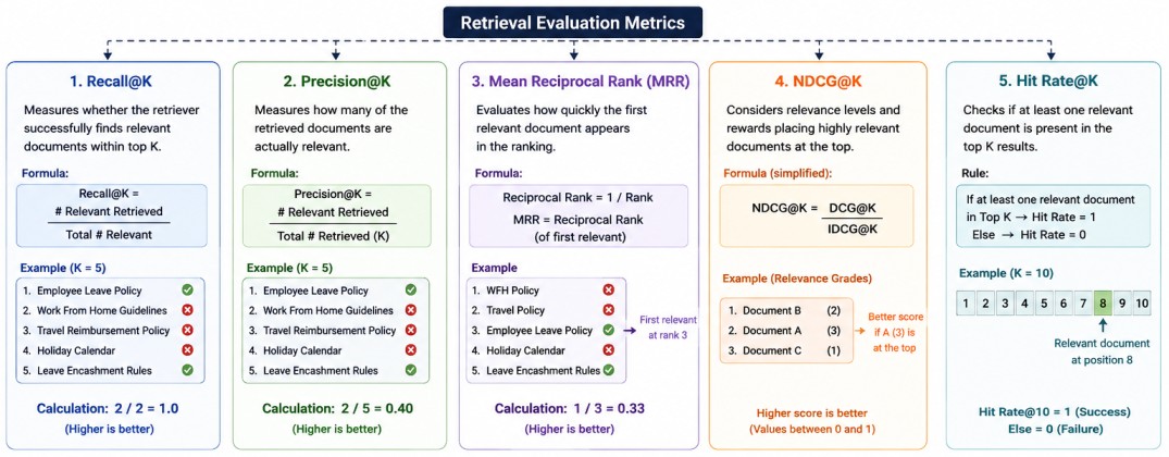
Retrieval Metrics
1. Recall@K
Recall@K measures whether the retriever successfully finds relevant documents within the top K results. Suppose the ground truth contains two relevant documents.Relevant Documents:
- Leave Encashment Rules
- Employee Leave Policy
Retrieved Documents:
- #1. Employee Leave Policy
- #2. Work From Home Guidelines
- #3. Travel Reimbursement Policy
- #4. Holiday Calendar
- #5. Leave Encashment Rules
Both relevant documents are present.
Formula:
Recall@K = Number of Relevant Documents Retrieved / Total Relevant DocumentsPython implementation
def recall_at_k(retrieved, relevant, k):
    top_k = retrieved[:k]

    retrieved_relevant = len(
        set(top_k).intersection(set(relevant))
    )

    return retrieved_relevant / len(relevant)


retrieved_docs = [
    "Employee Leave Policy",
    "WFH Policy",
    "Travel Policy",
    "Holiday Calendar",
    "Leave Encashment Rules"
]

relevant_docs = [
    "Employee Leave Policy",
    "Leave Encashment Rules"
]

print(recall_at_k(retrieved_docs, relevant_docs, 5))
Output:
1.0
2. Precision@K
While Recall focuses on finding relevant documents, Precision@K measures how many retrieved documents are actually relevant. Consider:Retrieved:
- #1. Employee Leave Policy
- #2. WFH Policy
- #3. Travel Policy
- #4. Holiday Calendar
- #5. Leave Encashment Rules
Only two documents are relevant.
- Leave Encashment Rules
- Employee Leave Policy
Formula:
Precision@K = Number of Relevant Documents / Total Retrieved DocumentsPython implementation:
def precision_at_k(retrieved, relevant, k):
    top_k = retrieved[:k]

    hits = len(
        set(top_k).intersection(set(relevant))
    )

    return hits / k

retrieved_docs = [
    "Employee Leave Policy",
    "WFH Policy",
    "Travel Policy",
    "Holiday Calendar",
    "Leave Encashment Rules"
]

relevant_docs = [
    "Employee Leave Policy",
    "Leave Encashment Rules"
]

print(
    precision_at_k(
        retrieved_docs,
        relevant_docs,
        5
    )
)
Output:
0.43. Mean Reciprocal Rank (MRR)
MRR evaluates how quickly the first relevant document appears.Retrieved:
- #1. WFH Policy
- #2. Travel Policy
- #3. Leave Encashment Rules
- #4. Holiday Calendar
Relevant:
- Leave Encashment Rules
- Employee Leave Policy
The first relevant document appears at rank 3.
Formula:
Reciprocal Rank = 1 / RankPython implementation:
def reciprocal_rank(retrieved, relevant):
    for rank, doc in enumerate(retrieved, start=1):
        if doc in relevant:
            return 1 / rank

    return 0

retrieved_docs = [
    "WFH Policy",
    "Travel Policy",
    "Employee Leave Policy",
    "Holiday Calendar",
    "Leave Encashment Rules"
]

relevant_docs = [
    "Employee Leave Policy",
    "Leave Encashment Rules"
]

print(
    reciprocal_rank(
        retrieved_docs,
        relevant_docs
    )
)
Output:
0.334. NDCG (Normalized Discounted Cumulative Gain)
In many real-world retrieval systems, not all relevant documents are equally important. Some documents may perfectly answer the user's question, while others may provide only partial information.Because of this, simply measuring whether a document is relevant is often insufficient. Instead, documents are assigned different relevance scores.
For example:
Document A → Highly Relevant (3)
Document B → Moderately Relevant (2)
Document C → Slightly Relevant (1)
NDCG is a ranking metric that rewards systems for placing highly relevant documents near the top of the results list. Documents appearing higher in the ranking contribute more to the score than documents appearing lower down.
Suppose the retriever produces the following ranking:
#1. Document B (2)
#2. Document A (3)
#3. Document C (1)
Although all relevant documents were retrieved, the ranking is not optimal because the most relevant document (Document A) appears in the second position rather than the first. Consequently, the NDCG score will be lower than the ideal ranking where Document A appears first.
DCG applies a logarithmic penalty to documents appearing lower in the ranking.
DCG = rel₁ + (rel₂ / log₂(2 + 1)) + (rel₃ / log₂(3 + 1)) + ...DCG = 2 + (3 / log₂(3)) + (1 / log₂(4))
= 2 + (3 / 1.585) + (1 / 2)
= 2 + 1.893 + 0.5
= 4.393
The ideal ranking places documents in descending order of relevance:
- #1. Document A (3)
- #2. Document B (2)
- #3. Document C (1)
Now calculate DCG for the ideal ordering:
IDCG = 3 + (2 / log₂(3)) + (1 / log₂(4))
= 3 + (2 / 1.585) + (1 / 2)
= 3 + 1.262 + 0.5
= 4.762
NDCG normalizes DCG by dividing it by the ideal DCG.
NDCG = DCG / IDCG
NDCG = 4.393 / 4.762 = 0.922
An NDCG score of 1.0 represents a perfect ranking, while values closer to 0 indicate poorer rankings.
Python Implementation
import math

def dcg(relevance_scores):
    score = 0

    for i, rel in enumerate(relevance_scores):
        if i == 0:
            score += rel
        else:
            score += rel / math.log2(i + 2)

    return score


def ndcg(relevance_scores):
    actual_dcg = dcg(relevance_scores)

    ideal_scores = sorted(
        relevance_scores,
        reverse=True
    )

    ideal_dcg = dcg(ideal_scores)

    return actual_dcg / ideal_dcg


# Ranking:
# Document B -> 2
# Document A -> 3
# Document C -> 1

scores = [2, 3, 1]

print(
    f"NDCG: {ndcg(scores):.3f}"
)
Output:
NDCG: 0.922A retrieval system that places highly relevant documents near the top will achieve a higher NDCG score than one that retrieves the same documents but ranks them poorly.
5. Hit Rate
Another simple yet highly practical metric used in production RAG (Retrieval-Augmented Generation) systems is Hit Rate.Unlike metrics such as Precision, Recall, or MRR, Hit Rate answers a very straightforward question: Was at least one relevant document retrieved within the top K results?
If the answer is yes, the retrieval is considered successful; otherwise, it is considered a failure. Because of its simplicity, Hit Rate is often used as a quick indicator of retrieval effectiveness.
Consider the following example. Suppose the retriever returns the top 10 documents for a query:
- #1. WFH Policy
- #2. Travel Policy
- #3. Security Guidelines
- #4. Holiday Calendar
- #5. Expense Policy
- #6. Training Manual
- #7. Employee Benefits
- #8. Leave Encashment Rules
- #9. Payroll Policy
- #10. IT Helpdesk Guide
Assume that Leave Encashment Rules is the only relevant document. Since at least one relevant document appears within the top 10 results, the query is considered a successful retrieval.
Formula (Single Query):
Hit Rate@K = 1 (if at least one relevant document is found in Top K) 0 (otherwise)- Query 1 → Hit
- Query 2 → Hit
- Query 3 → Miss
- Query 4 → Hit
- Query 5 → Miss
Formula:
Hit Rate = Number of Successful Queries / Total Number of QueriesThis means that the retriever successfully returned at least one relevant document for 60% of the evaluated queries.
Python Implementation (Single Query)
def hit_rate_at_k(
    retrieved_docs,
    relevant_docs,
    k
):
    top_k = retrieved_docs[:k]

    for doc in top_k:
        if doc in relevant_docs:
            return 1

    return 0


retrieved_docs = [
    "WFH Policy",
    "Travel Policy",
    "Security Guidelines",
    "Holiday Calendar",
    "Expense Policy",
    "Training Manual",
    "Employee Benefits",
    "Leave Encashment Rules",
    "Payroll Policy",
    "IT Helpdesk Guide"
]

relevant_docs = [
    "Leave Encashment Rules"
]

print(
    hit_rate_at_k(
        retrieved_docs,
        relevant_docs,
        10
    )
)
Output:
1Python Implementation (Multiple Queries)
def hit_rate(results):
    return sum(results) / len(results)


query_results = [
    1,  # Hit
    1,  # Hit
    0,  # Miss
    1,  # Hit
    0   # Miss
]

print(
    f"Hit Rate: {hit_rate(query_results):.2f}"
)
Output:
Hit Rate: 0.60Because of this, Hit Rate is often used alongside metrics such as MRR, NDCG, and Recall, which provide deeper insights into ranking quality.
End-to-End Retrieval Evaluation
While individual retrieval metrics such as Recall, Precision, and MRR help evaluate the effectiveness of the retriever, modern RAG (Retrieval-Augmented Generation) systems often perform end-to-end evaluation, where both the retrieval and generation stages are assessed together.The goal is to determine not only whether the correct information was retrieved but also whether the Large Language Model used that information correctly to generate the final answer.
For example, consider the question, "When was Spring Boot first released?" If the retriever successfully returns a document stating that "Spring Boot was initially released in April 2014" and the language model generates the answer "Spring Boot was first released in April 2014", then both the retrieval and generation stages are considered correct.
However, there can be situations where retrieval succeeds but generation fails. Suppose the same correct document is retrieved, but the language model responds with "Spring Boot was first released in 2015". In this case, the retriever has done its job correctly by providing accurate information, but the generation component has produced an incorrect answer.
End-to-end evaluation is valuable because it helps teams identify the true source of failures within a RAG pipeline. If the retrieved documents do not contain the necessary information, the issue lies in retrieval. If the correct information is retrieved but the final answer is still wrong, the problem lies in the generation stage.
This distinction is crucial for diagnosing system behavior and prioritizing improvements in production RAG applications.
What Are Re-Rankers?
A retriever is optimized for speed. It searches millions of documents and returns a relatively small set of candidates. However, the ranking produced by the retriever is not always optimal.A Re-Ranker is a secondary model that examines the retrieved documents and reorders them according to true semantic relevance.
The architecture typically looks like:
User Query → Retriever (e.g., Elasticsearch) → Top 100 Documents → Re-Ranker (e.g., rerank-english-v3.0) → Top 10 Documents → LLM
Why Retrievers Sometimes Rank Incorrectly
Suppose a user asks: How does Spring Boot auto-configuration work?A vector retriever might return:
- #1. Spring Framework Overview
- #2. Dependency Injection Concepts
- #3. Spring Boot Auto Configuration
- #4. Spring Security Basics
The correct document appears at position 3. This happens because embeddings capture general semantic similarity but may not fully understand the exact relationship between query and document.
A re-ranker analyzes each query-document pair more deeply and may reorder results as:
- #1. Spring Boot Auto Configuration
- #2. Spring Framework Overview
- #3. Dependency Injection Concepts
- #4. Spring Security Basics
Now the most relevant document appears first.
Cross-Encoder Re-Rankers
Most modern re-rankers use a Cross-Encoder architecture. A traditional embedding retriever processes query and document independently:Query → Embedding
Document → Embedding
Cosine Similarity
[Query] + [Document] → Transformer → Relevance ScoreExample
Query: How does Spring Boot auto-configuration work?Document A:
Spring Boot automatically configures beans based on
classpath dependencies.
Introduction to dependency injection.
Python Implementation
from sentence_transformers import CrossEncoder

# Load pre-trained Cross-Encoder model
model = CrossEncoder(
    "cross-encoder/ms-marco-MiniLM-L-6-v2"
)

query = "How does Spring Boot auto-configuration work?"

documents = [
    """Spring Boot automatically configures beans
    based on classpath dependencies.""",

    """Introduction to dependency injection.""",

    """Spring Security authentication and authorization.""",

    """Spring Boot auto-configuration uses
    @Conditional annotations to create beans
    automatically based on available dependencies."""
]

# Create query-document pairs
pairs = [
    [query, document]
    for document in documents
]

# Predict relevance scores
scores = model.predict(pairs)

# Combine documents and scores
results = list(zip(documents, scores))

# Sort by score descending
results.sort(
    key=lambda x: x[1],
    reverse=True
)

for document, score in results:
    print(f"Score: {score:.2f}")
    print(document)
    print("-" * 50)
Score: 8.77
Spring Boot auto-configuration uses
    @Conditional annotations to create beans
    automatically based on available dependencies.
--------------------------------------------------
Score: 4.29
Spring Boot automatically configures beans
    based on classpath dependencies.
--------------------------------------------------
Score: -7.21
Spring Security authentication and authorization.
--------------------------------------------------
Score: -11.33
Introduction to dependency injection.
--------------------------------------------------
This happens because the model evaluates the query and document together, allowing it to understand deeper semantic relationships rather than relying solely on vector similarity.
Re-Ranking using a Vector Database
candidate_docs = vector_store.similarity_search(
    query,
    k=100
)

ranked_docs = reranker.rank(
    query,
    candidate_docs
)

final_docs = ranked_docs[:5]
Conclusion
Without re-ranking, a retriever might return useful documents but place them in poor positions. Since only a limited number of documents can fit into an LLM prompt, ranking quality becomes extremely important.Re-rankers improve Precision, MRR, NDCG, answer quality, and context utilization. For this reason, most enterprise-grade RAG systems use a two-stage retrieval architecture where the retriever maximizes recall and the re-ranker maximizes ranking accuracy.