Because of this question-based structure, Decision Trees are easy to understand, explain, and visualize. They are used in classification tasks such as fraud detection, disease diagnosis, spam filtering, and churn prediction, as well as regression tasks such as price prediction or demand forecasting.
This article explains Decision Trees practically, including intuition, splitting logic, core mathematics, Python examples, strengths, limitations, and real-world usage.
What is a Decision Tree?
A Decision Tree is a supervised learning model that splits data into smaller groups by asking feature-based questions. Each internal node contains a decision rule, each branch represents an outcome of that rule, and each leaf node contains the final prediction.
The main goal of a Decision Tree is to split data so that each resulting group becomes as pure as possible. A pure group means the observations inside it mostly belong to one target class.
Suppose a node contains customers who both churn and stay. If splitting by complaint count creates one branch mostly churners and another mostly loyal customers, that split is valuable.
So the tree repeatedly asks: which question best separates the classes?
Root Node is the first and most important split, Internal Nodes are additional decision points, Branches represent outcomes such as yes/no or threshold results, and Leaf Nodes contain the final prediction or value.
The root node usually uses the feature that provides the best first separation.
At every node, the algorithm tests many candidate splits and selects the one that best improves purity. For numerical data, this may be thresholds such as:
Income < 50000
Age > 42
Usage Score < 0.31
Gini Impurity
One common metric used in classification trees is Gini Impurity. It helps the algorithm decide how good or bad a split is by measuring how mixed the target classes are inside a node. In simple terms, it answers the question: "If I randomly pick a record from this node, how likely is it that it belongs to the wrong class?"The formula is:
Gini = 1 − ∑i=1k pi2If a node contains only one class, then one probability is 1 and all others are 0. That gives:
Gini = 1 − 12 = 0Suppose a node has 50% class A and 50% class B. Then:
Gini = 1 − (0.52 + 0.52) = 0.5Now suppose a node has 80% class A and 20% class B:
Gini = 1 − (0.82 + 0.22) = 0.32During training, the Decision Tree tests many possible splits and chooses the one that creates child nodes with the lowest Gini Impurity. In other words, it prefers splits that separate the classes into purer groups.
So in practice, Gini = 0 indicates a perfectly pure node, Low Gini means the node mostly contains one class, and High Gini represents mixed classes.
Gini Impurity is useful because it gives a numerical score for how clean or mixed a group of data is, allowing a Decision Tree to automatically choose the best split at every step.
For example, imagine a bank wants to predict loan default. If one split creates:
Group A: 95% safe customers, 5% defaulters
Group B: 20% safe customers, 80% defaulters
then both groups are much cleaner than the original mixed dataset. Gini detects this and rewards that split.
Entropy and Information Gain
Another widely used criterion in Decision Trees is Entropy, a concept borrowed from information theory. Entropy measures the amount of uncertainty, randomness, or disorder inside a node. In simple terms, it tells us how mixed the target classes are and how difficult it is to make a confident prediction from that node.If almost all records in a node belong to one class, the node is clean and predictable, so entropy is low. If the classes are evenly mixed, the node is uncertain and entropy becomes high.
The mathematical formula is:
Entropy = − ∑i=1k pi log2(pi)
If a node contains only one class, entropy becomes 0, meaning perfect purity and no uncertainty. If two classes are split 50% and 50%, entropy becomes high because the model cannot clearly decide which class dominates.
For example, 100% Fraud Cases means Entropy = 0, 50% Fraud and 50% Safe results in High Entropy, and 80% Fraud with 20% Safe gives Medium Entropy.
The Decision Tree does not stop at measuring entropy. It uses entropy to find the best split through a metric called Information Gain. Information Gain measures how much uncertainty is removed after splitting a parent node into child nodes.
The formula is:
IG = Entropy(parent) − ∑ wj Entropy(childj)
If the child nodes become much cleaner than the parent node, Information Gain is high. If the split does little to improve purity, Information Gain is low.
For example, suppose a customer node contains mixed churners and loyal users. If splitting by complaint count creates one branch with mostly churners and another with mostly loyal users, entropy falls sharply. That split has high Information Gain and is considered valuable.
So in practice, Low Entropy indicates a pure node with an easy decision, High Entropy represents a mixed node with uncertain decisions, and High Information Gain means an excellent split that significantly reduces disorder.
This is why Decision Trees often choose the split that maximizes Information Gain—it helps the model grow branches that separate classes in the clearest possible way.
Simple Example
Suppose we want to predict loan default risk using features such as income and number of missed payments. A Decision Tree may automatically learn rules like:If Missed Payments > 2, the customer is classified as High Risk; else if Income < 30000, the customer is classified as Medium Risk; otherwise, the customer is classified as Low Risk.
This means customers with many missed payments are immediately flagged as risky, while customers with fewer missed payments are further evaluated using income. Lower income may indicate moderate repayment risk, while stable income with clean payment behavior suggests low risk.
The power of Decision Trees is that these rules are easy to read, explain, and justify to business teams, auditors, or managers. Unlike many black-box models, a tree clearly shows why a prediction was made. That is why Decision Trees are naturally interpretable and often trusted in domains such as banking, healthcare, and insurance.
Below is a practical example using scikit-learn to predict loan default from customer age and missed payment history.
from sklearn.tree import DecisionTreeClassifier
from sklearn.model_selection import train_test_split
from sklearn.metrics import accuracy_score
from sklearn.tree import plot_tree
import matplotlib.pyplot as plt
import numpy as np

# Features: age, missed_payments
X = np.array([
    [25, 1],
    [45, 0],
    [35, 3],
    [52, 0],
    [23, 4],
    [40, 1],
    [29, 2],
    [50, 0]
])

# Target:
# 0 = No Default
# 1 = Default
y = np.array([0, 0, 1, 0, 1, 0, 1, 0])

# Split dataset
X_train, X_test, y_train, y_test = train_test_split(
    X, y, test_size=0.25, random_state=42
)

# Build tree
model = DecisionTreeClassifier(
    max_depth=3,
    criterion="gini",
    random_state=42
)

# Train model
model.fit(X_train, y_train)

# Predict
pred = model.predict(X_test)

print("Predictions:", pred)
print("Accuracy:", accuracy_score(y_test, pred))

# Plot tree
plt.figure(figsize=(10, 6))
plot_tree(
    model,
    feature_names=["age", "missed_payments"],
    class_names=["No Default", "Default"],
    filled=True
)
plt.show()
Output:
Predictions: [0 0]
Accuracy: 1.0
One of the biggest strengths of Decision Trees is that the learned logic can be visualized.
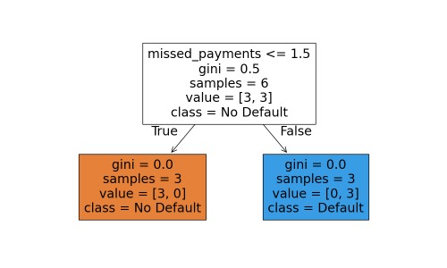
Decision Rules such as missed_payments > 2, Threshold Values as numerical split points, Class Distribution showing how many samples reach each node, and Leaf Predictions indicating the final default or no-default decision.
This transparency makes Decision Trees especially valuable when model explainability matters as much as prediction accuracy.
Decision Trees for Regression
Decision Trees are not limited to classification problems. They can also predict continuous numeric values using DecisionTreeRegressor. In this case, the goal is not to separate classes such as yes/no or fraud/not fraud, but to estimate values such as price, revenue, temperature, sales volume, or future demand.Instead of using metrics like Gini Impurity or Entropy, regression trees choose splits that reduce prediction error. A common objective is minimizing Mean Squared Error (MSE), which measures how far predictions are from actual values. The tree keeps splitting data into smaller groups where target values are more similar.
For example, in house price prediction, the tree may learn rules such as:
Area < 1200 sq f: Lower Price Range
Area ≥ 1200 sq ft and Location Score > 8: Higher Price Range
Else: Medium Price Range
Common use cases include house price estimation, sales forecasting, demand planning, insurance claim cost prediction, energy usage forecasting, and many business planning tasks.
Below is a practical example where we predict house prices using size and number of rooms.
from sklearn.tree import DecisionTreeRegressor, plot_tree
from sklearn.model_selection import train_test_split
from sklearn.metrics import mean_squared_error
import matplotlib.pyplot as plt
import numpy as np

# Features:
# [house_size_sqft, rooms]
X = np.array([
    [800, 2],
    [1000, 2],
    [1200, 3],
    [1500, 3],
    [1800, 4],
    [2000, 4],
    [2300, 5],
    [2600, 5]
])

# Target: House Price ($)
y = np.array([
    120000,
    150000,
    180000,
    220000,
    270000,
    310000,
    360000,
    420000
])

# Split dataset
X_train, X_test, y_train, y_test = train_test_split(
    X, y, test_size=0.25, random_state=42
)

# Build regression tree
model = DecisionTreeRegressor(
    max_depth=3,
    random_state=42
)

# Train model
model.fit(X_train, y_train)

# Predict
pred = model.predict(X_test)

print("Predictions:", pred)
print("Actual:", y_test)

# Error
mse = mean_squared_error(y_test, pred)
print("MSE:", mse)

# Plot regression tree
plt.figure(figsize=(12, 7))
plot_tree(
    model,
    feature_names=["house_size_sqft", "rooms"],
    filled=True,
    rounded=True
)
plt.title("Decision Tree Regressor")
plt.show()
random_state=42 sets the starting seed for the model’s internal random number generator. This means any random operations, such as how data is split or how ties are resolved, happen the same way each time, so you get the same results whenever the code runs.
Output:
Predictions: [120000. 270000.]
Actual: [150000 310000]
MSE: 1250000000.0
MSE = 1,250,000,000 means the model's predictions still have significant error from actual house prices. In this case, predictions are off by roughly $35,355 on average (RMSE).
Prediction quality can be improved by using more training data, adding useful features such as location and house age, tuning tree parameters, or using stronger models like Random Forest or Gradient Boosting.

For example, a house with 1600 sq ft and 3 rooms follows the path of conditions and may reach a leaf predicting $220,000. This makes the model highly interpretable because users can clearly see how each prediction was made.
Conclusion
Decision Trees turn prediction into a sequence of understandable questions. Mathematically, they choose splits that maximize purity using metrics such as Gini or Entropy. Practically, they offer one of the clearest bridges between statistics and human decision logic.Decision Trees are highly interpretable, require little preprocessing, handle nonlinear relationships, work with numerical and categorical logic, and naturally capture feature interactions. They do not require feature scaling like K-Means or Logistic Regression often does. They are excellent when explainability matters.
Single trees can overfit training data, especially when grown too deep. They may become unstable because small data changes can create different trees. They can also underperform compared with ensemble methods. This is why Random Forest and Gradient Boosting often outperform a single tree.
Although ensemble methods often outperform single trees, understanding Decision Trees is essential because they form the foundation of many of the most powerful models used today.