This article explains Logistic Regression in a practical way, covering classification intuition, probability modeling, training logic, decision boundaries, and implementation using Python.
Suppose we want to predict whether a student will pass an exam based on study hours. If we apply Linear Regression directly, the predictions may be values such as 1.3 or -0.4, which do not make sense as class labels or probabilities. Classification problems require outputs constrained between 0 and 1 so they can represent probabilities. This is the central reason Logistic Regression exists.
Core Idea of Logistic Regression
Logistic Regression first computes a weighted linear combination of input features, then transforms that score into a probability using the sigmoid function.z = b + w1x1 + w2x2 + ⋯ + wnxn
The raw score z can be any real number. It is then converted into probability form:
σ(z) = 1/1 + e-z
The sigmoid compresses outputs into the range from 0 to 1. Values near 1 indicate strong confidence in the positive class, while values near 0 indicate confidence in the negative class.
Once a probability is produced, a threshold is applied. The most common threshold is 0.5. If the predicted probability is greater than or equal to 0.5, the model predicts class 1. Otherwise, it predicts class 0.
For example, if fraud probability is 0.87, the transaction may be labeled suspicious. If churn probability is 0.12, the customer may be labeled likely to stay.
Each coefficient (w) in Logistic Regression measures how a feature influences the log-odds of the positive outcome. In practical terms, positive coefficients increase probability, while negative coefficients reduce probability. Larger magnitudes imply stronger influence.
This interpretability is one reason Logistic Regression remains popular in regulated industries where explanations matter.
Training the Model
Unlike Linear Regression, Logistic Regression does not use Mean Squared Error (MSE) as its main loss function. Instead, it uses log loss, also known as cross-entropy loss. This loss function is designed for classification problems and gives a high penalty when the model makes a wrong prediction with high confidence.L = -1/n ∑i=1n [ yi log(ŷi) + (1 - yi) log(1 - ŷi) ]
Here:
- yi = actual class label (0 or 1)
- ŷi = predicted probability
- n = total number of training examples
The goal of training is to find the best coefficients (weights) that minimize this loss. To do this, optimization algorithms such as gradient descent or other advanced solvers are used.
Suppose we want to predict whether a user will buy a product based on the time spent on a website. Usually, users who spend more time are more likely to make a purchase. Logistic Regression learns this relationship as a smooth S-shaped curve, instead of an unrestricted straight line.
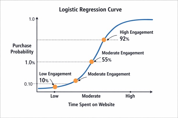
- Low engagement may give a probability near 0.10
- Moderate engagement may give a probability near 0.55
- High engagement may give a probability near 0.92
This makes Logistic Regression useful because it provides realistic probabilities between 0 and 1.
Implementation with sklearn
In practice, scikit-learn provides a robust implementation.import numpy as np
from sklearn.linear_model import LogisticRegression
X = np.array([[1], [2], [3], [4], [5], [6]])
y = np.array([0, 0, 0, 1, 1, 1])
model = LogisticRegression()
model.fit(X, y)
print("Coefficient:", model.coef_[0][0])
print("Intercept:", model.intercept_[0])
- X contains the input values: 1, 2, 3, 4, 5, 6
- y contains the target labels: first three belong to class 0, last three belong to class 1
- LogisticRegression() creates the model
- model.fit(X, y) trains the model by learning the relationship between X and y
After training:
- model.coef_[0][0] gives the learned coefficient (slope), showing how strongly X affects the prediction
- model.intercept_[0] gives the intercept (bias term)
The model learns that lower values of X are linked to class 0, while higher values are linked to class 1. It then uses the sigmoid function to convert the result into probabilities.
Possible output:
Coefficient: 1.1206952510393666
Intercept: -3.9223038967769632prob = model.predict_proba([[4]])[0][1]
label = model.predict([[4]])[0]
print("Probability:", round(prob, 3))
print("Class:", label)
prob = model.predict_proba([[4]])[0][1] calculates the probability that the input value 4 belongs to class 1 using the trained Logistic Regression model. [0] selects the first (and only) prediction row and [1] selects the second value, which is the probability of class 1.
If the probability is greater than the decision threshold (usually 0.5), the model predicts class 1; otherwise, it predicts class 0.
Possible output:
Probability: 0.637
Class: 1
This is why Logistic Regression is considered a linear classifier: the boundary is linear in feature space.
Multiple Features
Logistic Regression is not limited to a single input variable. It can use multiple features at the same time to make better predictions. Instead of relying on only one factor, the model studies several variables together and uses all of them to estimate the final probability.For example, suppose a company wants to predict whether a customer will churn (leave the service). Instead of using only one feature, it can use:
- Monthly usage
- Contract length
- Number of complaints
- Support calls
- Subscription age
Each feature gets its own weight (coefficient). Features that increase churn probability get positive influence, while features that reduce churn probability get negative influence.
The model calculates:
z = b + w1x1 + w2x2 + w3x3 + ... + wnxn
Then it applies the sigmoid function to convert this score into a probability between 0 and 1.
Python Example:
import numpy as np
from sklearn.linear_model import LogisticRegression

# Features:
# [monthly_usage, contract_length, complaints]
X = np.array([
    [80, 12, 0],
    [20, 2, 3],
    [60, 10, 1],
    [15, 1, 4],
    [75, 11, 0],
    [30, 3, 2]
])

# Target:
# 0 = Stay, 1 = Churn
y = np.array([0, 1, 0, 1, 0, 1])

# Train model
model = LogisticRegression()
model.fit(X, y)

# Predict for new customer
new_customer = [[25, 2, 3]]

prob = model.predict_proba(new_customer)[0][1]
label = model.predict(new_customer)[0]

print("Churn Probability:", round(prob, 3))
print("Prediction:", label)
- Low monthly usage = 25
- Short contract = 2 months
- 3 complaints
These signals may indicate churn risk. The model combines all three features and predicts the probability that the customer will leave. If output is:
Churn Probability: 0.998
Prediction: 1
Regularization
To reduce overfitting, Logistic Regression often uses a technique called regularization. Overfitting happens when a model learns the training data too closely, including noise or random patterns, and then performs poorly on new unseen data. Regularization helps prevent this by discouraging very large coefficient values and encouraging a simpler model that generalizes better.In Logistic Regression, each feature receives a weight (coefficient) that affects predictions. If some coefficients become extremely large, the model may become too sensitive to small changes in input values. Regularization adds a penalty during training, so the model tries to do two things at the same time:
- Fit the training data well
- Keep the coefficients reasonably small and stable
This often leads to better real-world performance. The two most common types are L1 regularization and L2 regularization.
- L1 Regularization shrinks some coefficients all the way to zero. This effectively removes less useful features, so it is often helpful for feature selection.
- L2 Regularization reduces coefficients gradually toward smaller values, but usually does not make them exactly zero. It is commonly used when we want a stable and balanced model.
For example, in spam detection with thousands of word-based features, or customer churn prediction with many behavioral signals, regularization can improve test accuracy and make the model more reliable.
The strength of regularization is controlled by a parameter that must be tuned carefully. Too little regularization may still allow overfitting, while too much may oversimplify the model and reduce accuracy. The best value is usually found using cross-validation.
Evaluation Metrics
Classification models should not be judged by accuracy alone, especially when the dataset is imbalanced. Accuracy measures the percentage of correct predictions, but it can be misleading when one class is much more common than the other.For example, if only 1% of transactions are fraudulent, a model that predicts every transaction as legitimate would still achieve 99% accuracy while completely failing to detect fraud.
Because of this, engineers use other metrics that give a clearer picture of model performance. The most common are precision, recall, F1-score, ROC-AUC, and PR-AUC.
Precision
Precision tells us how many predicted positive cases were actually correct.
Example:
If the model marks 100 transactions as fraud, and 80 are truly fraud:
Precision = 80%
High precision is important when false alarms are costly.
Recall
Recall tells us how many actual positive cases the model successfully found.
Example:
If there were 100 fraudulent transactions, and the model detected 90:
Recall = 90%
High recall is important when missing positive cases is risky.
F1-score
F1-score combines precision and recall into one balanced metric. It is useful when both false positives and false negatives matter.
ROC-AUC
ROC-AUC measures how well the model separates the two classes across many decision thresholds. A higher value means better class separation.
PR-AUC
PR-AUC (Precision-Recall Area Under Curve) is often more useful for highly imbalanced datasets because it focuses on positive-class detection.
Which Metric Matters Most?
The best metric depends on the business problem:
- Fraud Detection: High recall may be preferred so fraud cases are not missed.
- Medical Screening: High recall is often important to catch possible patients.
- Marketing Campaigns: High precision may matter more to avoid wasting budget.
- Spam Detection: Precision and recall may both be important.
A skilled engineer does not ask for one universal best metric. Instead, they choose the metric that matches the real cost of mistakes and the actual goal of the system.
Example: Customer Churn Prediction
Suppose a telecom company wants to predict whether a customer will leave the service. We use three features:• Monthly bill
• Number of complaints
• Contract length
import pandas as pd
import matplotlib.pyplot as plt
from sklearn.model_selection import train_test_split
from sklearn.linear_model import LogisticRegression
from sklearn.metrics import classification_report, confusion_matrix, roc_auc_score

# Sample dataset
data = pd.DataFrame({
    "monthly_bill": [20, 25, 30, 35, 40, 45, 50, 55, 60, 65, 70, 75],
    "complaints": [0, 0, 1, 0, 1, 1, 2, 2, 3, 3, 4, 4],
    "contract_months": [24, 22, 20, 18, 16, 14, 12, 10, 8, 6, 4, 2],
    "churn": [0, 0, 0, 0, 0, 0, 1, 1, 1, 1, 1, 1]
})

X = data[["monthly_bill", "complaints", "contract_months"]]
y = data["churn"]

# Split dataset
X_train, X_test, y_train, y_test = train_test_split(
    X, y, test_size=0.3, random_state=42
)

# Train model
model = LogisticRegression()
model.fit(X_train, y_train)

# Predictions
pred = model.predict(X_test)
prob = model.predict_proba(X_test)[:, 1]

print("Predictions:", pred)
print("Probabilities:", prob.round(3))
print(confusion_matrix(y_test, pred))
print(classification_report(y_test, pred))
print("ROC-AUC:", round(roc_auc_score(y_test, prob), 3))
• y contains the target values: 0 = Stay & 1 = Churn
• train_test_split() divides the data into training and testing sets.
• model.fit() trains the Logistic Regression model.
• predict() gives final class labels.
• predict_proba() gives churn probabilities.
Possible Output
Predictions: [1 1 0 1]
Probabilities: [1. 1. 0. 1.]
[[1 0]
 [0 3]]
              precision    recall  f1-score   support

           0       1.00      1.00      1.00         1
           1       1.00      1.00      1.00         3

    accuracy                           1.00         4
   macro avg       1.00      1.00      1.00         4
weighted avg       1.00      1.00      1.00         4

ROC-AUC: 1.0
The model predicted 4 test customers:
- 3 customers may churn
- 1 customer may stay
Probabilities: [1. 1. 0. 1.]
These are predicted probabilities for class 1 (churn). The model is highly confident in these predictions.
Confusion Matrix:
[[1 0]
 [0 3]]
- 1 actual non-churn customer was predicted correctly
- 3 actual churn customers were predicted correctly
- No mistakes were made
ROC-AUC = 1.0
This means perfect separation between churn and non-churn customers in this test set.
These results look perfect, but the dataset is very small. Only a few test samples were used, so this does not guarantee real-world performance. Larger datasets and proper validation are needed before trusting the model fully.
Probability Curve
If we plot churn probability against monthly bill (keeping other features fixed), Logistic Regression usually creates an S-shaped curve.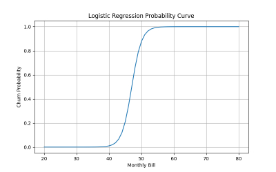
- Higher monthly bills may increase churn risk sharply after a threshold
This shows why probability outputs are valuable. Businesses can prioritize decisions instead of treating every customer the same.
Conclusion
Logistic Regression is one of the foundational algorithms of classification. It transforms linear signals into probabilities using the sigmoid function, creates clear decision boundaries, and offers interpretable predictions with strong practical value.Although more advanced models exist, Logistic Regression remains timeless because many real problems reward clarity, speed, and reliable probability estimates. When used thoughtfully, it is far more powerful than its simplicity suggests.