Linear Regression attempts to model the relationship between one or more input variables and a continuous output value. If house size increases, price may increase. If advertising spend rises, sales may improve. If years of experience increase, salary may rise. The model learns these relationships mathematically and uses them for prediction.
This article explains Linear Regression practically, including the mathematical intuition, how to build it from scratch, and how to use it efficiently with scikit-learn.
Core Idea of Linear Regression
Linear Regression fits a straight-line relationship between variables. In the simplest single-variable case, the model estimates a line where predictions are made using an intercept and slope.y=mx+b
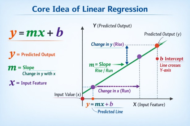
In machine learning language, slope values become coefficients, and the intercept becomes the bias term.
In Machine Learning, coefficients are the weights assigned to each input feature that show how much that feature influences the prediction. A larger coefficient means stronger impact.
The bias term is a constant value added to the model output, allowing the prediction to shift up or down independently of input features. It helps the model fit data more accurately.
Example (Linear Regression):
Prediction = (coefficient × feature) + bias
Multiple Linear Regression
Real-world problems often involve many variables rather than one. House price may depend on size, bedrooms, location score, age, and neighborhood demand. In such cases, Linear Regression extends naturally to multiple inputs.y = b + w1·x1 + w2·x2 + w3·x3 + ⋯ + wn·xn
Each coefficient measures the contribution of one feature while holding others constant.
How the Model Learns
The model must choose coefficient values that minimize prediction error. It does this by comparing predicted values with actual target values and finding parameters that reduce total loss. The most common loss function is Mean Squared Error, where larger mistakes are penalized more heavily.MSE = 1/n ∑i=1n (yi - ŷi)2
The lower the error, the better the fitted regression line.
Linear Regression from Scratch
To understand the algorithm deeply, it is useful to implement it manually using gradient descent. Gradient descent starts with random parameter values and improves them step by step by moving in the direction that reduces loss.import numpy as np
# Simple Linear Regression Example
# Study Hours -> Exam Marks
X = np.array([1, 2, 3, 4, 5], dtype=float) # Input feature
y = np.array([45, 50, 55, 60, 65], dtype=float) # Actual output
# Initialize weight and bias
w = 0.0
b = 0.0
# Learning rate and training loops
lr = 0.01
epochs = 1000
n = len(X)
# Gradient Descent Training
for _ in range(epochs):
y_pred = w * X + b
dw = (-2 / n) * np.sum(X * (y - y_pred))
db = (-2 / n) * np.sum(y - y_pred)
w -= lr * dw
b -= lr * db
# Final model values
print("Weight:", round(w, 2))
print("Bias:", round(b, 2))
Possible output:
Weight: 5.34
Bias: 38.79
y=5.34x+38.79
Which matches the pattern in the training data.
Once coefficients are learned, prediction becomes simple.
# Predict new value
x_new = 6  # 6 study hours
prediction = w * x_new + b

print("Predicted Marks:", round(prediction, 2))
Possible output:
Predicted Marks: 70.8Using Linear Regression with sklearn
While building from scratch teaches fundamentals, production work usually uses scikit-learn for speed, reliability, and convenience.import numpy as np
from sklearn.linear_model import LinearRegression
# Study Hours -> Exam Marks
X = np.array([1, 2, 3, 4, 5], dtype=float).reshape(-1, 1) # Input feature
y = np.array([45, 50, 55, 60, 65], dtype=float) # Actual output
# Create model
model = LinearRegression()
# Train model
model.fit(X, y)
# Show learned values
print("Weight (Coefficient):", round(model.coef_[0], 2))
print("Bias (Intercept):", round(model.intercept_, 2))
Possible output:
Weight (Coefficient): 5.0
Bias (Intercept): 40.0# Predict marks for 6 study hours
x_new = np.array([[6]])
prediction = model.predict(x_new)
print("Predicted Marks:", round(prediction[0], 2))
Possible output:
Predicted Marks: 70.0Evaluating Performance
Regression models are commonly evaluated using Mean Absolute Error, Mean Squared Error, Root Mean Squared Error, and R² Score.The R² score measures how much variance in the target is explained by the model.
R2 = 1 - SSres/SStot
Values closer to 1 generally indicate stronger fit.
Linear Regression performs best when the relationship between features and target is reasonably linear, errors are not strongly patterned, features are not excessively collinear, and extreme outliers are limited.
These assumptions are often approximations rather than rigid laws, but violating them can reduce reliability.
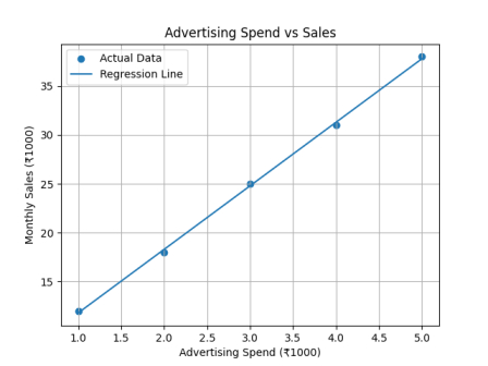
Real-World Example
Suppose a company wants to predict monthly sales based on advertising spend. If past data shows that increasing marketing budget usually increases sales in a nearly straight-line pattern, Linear Regression can model that relationship.It fits a line:
Sales = m × Advertising Spend + b
Where:
m = how much sales increase for every extra ₹1 spent on ads
b = base sales even with zero advertising spend
Example Historical Data
| Advertising Spend (₹1000) | Monthly Sales (₹1000) |
|---|---|
| 1 | 12 |
| 2 | 18 |
| 3 | 25 |
| 4 | 31 |
| 5 | 38 |
Sales = 6.5 × Ad Spend + 5.3
This means:
Every extra ₹1000 in advertising increases sales by about ₹6500
Even with no ads, expected sales are about ₹5300
Prediction Example
If company spends ₹6000 on ads:Sales = 6.5 × 6 + 5.3 = 44.3
Predicted monthly sales ≈ ₹44, 300
import numpy as np
import matplotlib.pyplot as plt
from sklearn.linear_model import LinearRegression

# Advertising Spend (₹1000)
X = np.array([1, 2, 3, 4, 5]).reshape(-1, 1)

# Monthly Sales (₹1000)
y = np.array([12, 18, 25, 31, 38])

# Train model
model = LinearRegression()
model.fit(X, y)

# Predictions for line
y_pred = model.predict(X)

# Print equation values
print("Slope:", round(model.coef_[0], 2))
print("Intercept:", round(model.intercept_, 2))

# Predict for ₹6000 ad spend
new_spend = np.array([[6]])
prediction = model.predict(new_spend)
print("Predicted Sales:", round(prediction[0], 2), "₹1000")

# Plot graph
plt.scatter(X, y, label="Actual Data")
plt.plot(X, y_pred, label="Regression Line")
plt.xlabel("Advertising Spend (₹1000)")
plt.ylabel("Monthly Sales (₹1000)")
plt.title("Advertising Spend vs Sales")
plt.legend()
plt.grid(True)
plt.show()
Output:
Slope: 6.5
Intercept: 5.3
Predicted Sales: 44.3 ₹1000
Evaluating Performance
After training a Linear Regression model, we need to check how well it predicts monthly sales. Common regression evaluation metrics are: - MAE (Mean Absolute Error)- MSE (Mean Squared Error)
- RMSE (Root Mean Squared Error)
= R² Score
Model Predictions
Suppose the trained regression line predicts:| Ad Spend | Actual Sales | Predicted Sales |
|---|---|---|
| 1 | 12 | 11.8 |
| 2 | 18 | 18.3 |
| 3 | 25 | 24.7 |
| 4 | 31 | 31.2 |
| 5 | 38 | 37.6 |
1. Mean Absolute Error (MAE)
Average of absolute prediction errors.MAE = (|12-11.8| + |18-18.3| + |25-24.7| + |31-31.2| + |38-37.6|) / 5
MAE ≈ 0.28
On average, predictions are off by ₹280
2. Mean Squared Error (MSE)
Squares errors before averaging.MSE = [(0.2² + 0.3² + 0.3² + 0.2² + 0.4²)] / 5
MSE ≈ 0.084
Larger mistakes get penalized more.
3. Root Mean Squared Error (RMSE)
Square root of MSE.RMSE = √MSE
RMSE ≈ 0.29
Typical prediction error is about ₹290
4. R² Score
Measures how much variation in sales is explained by advertising spend.R² = 1 - (SSres / SStot)
Where:
SSres = Sum of squared residual errors
SStot = Total variance in actual sales
For this example:
R² ≈ 0.999
About 99.9% of sales variation is explained by ad spend.
Python Code
import numpy as np
from sklearn.linear_model import LinearRegression
from sklearn.metrics import mean_absolute_error, mean_squared_error, r2_score

# Data
X = np.array([1, 2, 3, 4, 5]).reshape(-1, 1)
y = np.array([12, 18, 25, 31, 38])

# Train model
model = LinearRegression()
model.fit(X, y)

# Predict
y_pred = model.predict(X)

# Metrics
mae = mean_absolute_error(y, y_pred)
mse = mean_squared_error(y, y_pred)
rmse = np.sqrt(mse)
r2 = r2_score(y, y_pred)

print("MAE :", round(mae, 2))
print("MSE :", round(mse, 2))
print("RMSE:", round(rmse, 2))
print("R² Score:", round(r2, 3))
MAE : 0.24
MSE : 0.06
RMSE: 0.24
R² Score: 0.999
1. Check If Model Is Good Enough
For our example:
- Low MAE / RMSE - predictions are close to actual sales
- High R² - advertising spend explains sales well
Conclusion: The model is performing well.
2. Use Model for Future Prediction
Now predict sales for new ad budgets.
Example:
- ₹6000 ad spend - predicted sales
- ₹8000 ad spend - predicted sales
new_data = np.array([[6], [8]])
predictions = model.predict(new_data)
print(predictions)
Helps plan future marketing budgets.
3. Business Decision Making
Use results to answer:
- Is increasing ad spend worth it?
- How much extra revenue comes from ₹1000 more ads?
What budget gives target sales?
4. Check Residual Errors
Compare:
- Actual Sales - Predicted Sales
If errors show patterns, Linear Regression may not be ideal. Then try advanced models.
5. Improve the Model
If performance is weak:
Add more features (season, price, competitors, location)
- Remove outliers
- Collect more data
- Try Polynomial Regression
- Try Random Forest / XGBoost
6. Deploy the Model
Use it in:
- Excel dashboard
- Website form
- Business analytics tool
- Marketing budget planner
Real Workflow
Train Model → Evaluate Metrics → Predict Future → Improve Model → Use in Business
For Our Example
Since R² is very high, the next logical step is: Use the model to predict future monthly sales for different advertising budgets.
Conclusion
Linear Regression is one of the foundational tools of machine learning. It combines elegant mathematics, practical usefulness, and transparent interpretation. Building it from scratch teaches optimization and loss minimization, while using scikit-learn enables efficient real-world deployment.
Many modern systems use complex models, yet Linear Regression remains timeless because clarity is often as valuable as complexity. When a straight line captures reality well enough, it is difficult to beat.
new_data = np.array([[6], [8]])
predictions = model.predict(new_data)
print(predictions)