Despite the emergence of advanced algorithms such as Gradient Boosting, XGBoost, LightGBM, CatBoost, Deep Neural Networks, and Large Language Models (LLMs), Random Forest continues to be widely used in production systems because of its excellent balance of accuracy, robustness, interpretability, scalability, fault tolerance, and ease of tuning.
Boosting is a machine learning technique that combines multiple weak models (usually small decision trees) sequentially to create one highly accurate strong model. Each new model focuses specifically on correcting the errors made by the previous ones.
1. Gradient Boosting
Gradient Boosting is an ensemble learning technique that builds Decision Trees sequentially, where each new tree attempts to correct the errors made by previous trees. Unlike Random Forest, which reduces variance through averaging, Gradient Boosting primarily reduces bias and often achieves higher predictive accuracy on structured data.
Ensemble learning is a machine learning technique that combines multiple individual models (often called "base models" or "weak learners") to create a single, highly accurate, and robust predictive model. By aggregating predictions, ensembles minimize errors and prevent overfitting.
2. XGBoost (Extreme Gradient Boosting)
XGBoost is an optimized implementation of Gradient Boosting that introduces regularization, parallel processing, tree pruning, and efficient handling of sparse data. It became the dominant algorithm in machine learning competitions because of its excellent performance, scalability, and robustness.
3. LightGBM
LightGBM (Light Gradient Boosting Machine), developed by Microsoft, is a highly optimized Gradient Boosting framework designed for large-scale datasets. It uses histogram-based learning and leaf-wise tree growth, making it significantly faster and more memory-efficient than traditional boosting implementations.
4. CatBoost
CatBoost, developed by Yandex, is a Gradient Boosting framework specifically designed to handle categorical features efficiently without extensive preprocessing. It reduces prediction shift and often delivers strong performance with minimal hyperparameter tuning.
Prediction shift is a mismatch between the distribution of a model's training labels and its test-time predictions, usually caused by changes in the real-world input features over time (covariate shift). It results in the model making biased, inaccurate predictions because the live data no longer matches what it learned during training.
Covariate shift occurs when the distribution of a model’s input features changes between the training phase and production, but the underlying relationship between those features and the target label remains exactly the same.
5. Deep Neural Networks (DNNs)
Deep Neural Networks are machine learning models composed of multiple hidden layers that learn hierarchical representations from data. They excel in complex tasks such as image recognition, speech processing, natural language understanding, and recommendation systems where large volumes of data are available.
6. Large Language Models (LLMs) Large Language Models are extremely large transformer-based neural networks trained on vast amounts of text data to understand and generate human language. Models such as OpenAI GPT, Google Gemini, and Anthropic Claude can perform reasoning, summarization, coding, translation, question answering, and many other language-related tasks through prompt-based interaction.
From Decision Trees to Random Forest
Before understanding Random Forest, it is important to understand how an individual Decision Tree works.A Decision Tree recursively partitions data into smaller and smaller subsets by selecting the best possible split at each node.
The goal of every split is to create child nodes that are as pure as possible, meaning that records belonging to the same class are grouped together. Suppose we have the following dataset:
Age    Income    Buy Product
25     50000     Yes
30     70000     Yes
45     90000     No
50     85000     No
Age < 35
Age < 40

Income < 75000
Income < 80000
Age < 35

Left Node:
25 → Yes
30 → Yes

Right Node:
45 → No
50 → No
- Maximum tree depth reached
- Minimum samples required for a split
- Completely pure leaf nodes
The quality of a split is typically measured using metrics such as Gini Impurity or Entropy, which quantify how mixed the classes are within a node. The split that achieves the largest impurity reduction is chosen.
Once the tree has been constructed, predictions are made by traversing the tree from the root node to a leaf node based on feature values.
For example, a customer churn prediction tree may create rules such as:
IF monthly_spend > 1000
   AND contract_type = monthly
THEN
   churn = Yes
ELSE
   churn = No
However, they also suffer from a major limitation known as high variance. A small change in the training dataset can produce a completely different tree structure. As a result, Decision Trees often memorize noise and overfit the training data.
Random Forest was specifically designed to overcome these limitations. Instead of relying on a single Decision Tree, it builds hundreds or thousands of diverse trees and combines their predictions, significantly improving stability, robustness, and generalization performance.
Understanding "Random Forest"
Random Forest belongs to a category called Ensemble Learning. The central principle of ensemble learning is that multiple weak or moderately strong models can collectively create a much stronger model.The intuition is simple. "If one doctor diagnoses a disease, the diagnosis may be incorrect. If one hundred independent doctors provide diagnoses and a majority agree, the probability of a correct diagnosis increases significantly."
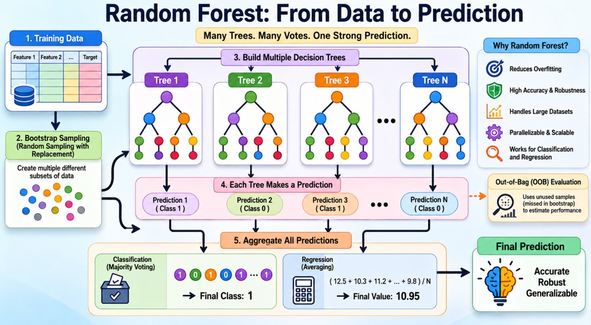
Dataset | Decision Tree | Prediction Dataset | | | | | | T1 T2 T3 T4 T5 Tn | | | | | Aggregation | Final Prediction The Two Sources of Randomness
Random Forest derives its power from introducing randomness in two independent ways.1. The first source is Bootstrap Sampling.
2. The second source is Random Feature Selection.
Together, these mechanisms ensure that individual trees are sufficiently different from one another. This diversity is critical because averaging highly correlated trees provides little benefit.
1. Bootstrap Sampling (Bagging)
Random Forest uses a technique called Bootstrap Aggregating, commonly known as Bagging.Suppose a dataset contains 100,000 records. For each tree, the algorithm randomly samples 100,000 records with replacement. Sampling with replacement means:
Original Dataset:
- Record 1
- Record 2
- Record 3
- Record 4
- Record 5
Bootstrap Sample:
- Record 1
- Record 1
- Record 3
- Record 5
- Record 5
Some records may appear multiple times. Some records may not appear at all. Each tree therefore learns from a slightly different dataset.
2. Random Feature Selection
In a normal Decision Tree, every feature is evaluated when selecting the best split.Suppose we have:
- Age
- Salary
- Location
- Education
- Experience
- Credit Score
- Transaction Count
A traditional tree examines all features at every split. Random Forest instead randomly chooses a subset:
Split 1:
- Age Salary
- Experience
Split 2:
- Location
- Education
- Credit Score
This prevents all trees from repeatedly selecting the same dominant features and increases diversity across the forest.
Random Forest Training and Prediction
Now that we understand bootstrap sampling and random feature selection, we can examine the complete Random Forest training process.Suppose we have a dataset containing 100,000 customer records and 50 features.
Training Phase
For each tree in the forest, the following steps are performed:Step 1: Draw a bootstrap sample from the original dataset.
Step 2: Create a new Decision Tree.
Step 3: At each node, randomly select a subset of available features.
Step 4: Evaluate possible splits using Gini Impurity or Entropy.
Step 5: Choose the best split.
Step 6: Repeat recursively until stopping criteria are reached.
Step 7: Store the trained tree.
Repeat the entire process for all trees in the forest.
Each tree sees a different bootstrap sample and evaluates different subsets of features, making every tree slightly different.
Prediction Phase
After training is complete, predictions are generated by all trees and then aggregated. For a classification problem:
Tree1 → Fraud
Tree2 → Genuine
Tree3 → Fraud
Tree4 → Fraud
Tree5 → Genuine
Tree1 → 100
Tree2 → 120
Tree3 → 110
Tree4 → 115
The aggregation step is what makes Random Forest powerful. Individual trees may make mistakes, but averaging or voting across many trees significantly reduces variance and improves generalization.
Mathematical Intuition
One of the most common questions is: Why does Random Forest work so well? The answer lies in the Bias-Variance Tradeoff.Prediction error can be decomposed as:
Total Error = Bias² + Variance + Irreducible Error
Bias: The error introduced by approximating a complex real-world problem with a model that is too simple. High bias causes the model to underfit, meaning it misses important trends and performs poorly on both training and test data.Decision Trees typically exhibit Low Bias High Variance. They can model complex patterns but are highly sensitive to data fluctuations.
Variance: The model's sensitivity to small fluctuations or noise in the training dataset. High variance causes the model to overfit, meaning it memorizes the training data perfectly but fails to generalize to new, unseen data.
Irreducible Error: The inherent noise or randomness in a dataset that cannot be removed by any model, no matter how perfect. It is caused by unmeasured variables, faulty data collection, or natural randomness.
Random Forest maintains low bias while dramatically reducing variance through averaging. If multiple independent trees have prediction variance:
Variance(Tree) = σ² Variance(Forest) ≈ σ² / N Out-of-Bag Error
One of the most elegant aspects of Random Forest is the concept of Out-of-Bag (OOB) Validation.Due to bootstrap sampling, approximately 63.2% records are included in a bootstrap sample. The remaining 36.8% records are excluded. These excluded records become Out-of-Bag samples.
Since a tree has never seen its OOB samples during training, they can be used for validation. This provides an internal estimate of model performance without requiring a separate validation dataset.
Why is OOB error useful?
Because it reduces the need for expensive cross-validation and provides a nearly unbiased estimate of generalization performance.
Feature Importance
One of the major advantages of Random Forest is its ability to estimate the importance of individual features automatically. In many enterprise applications, understanding why a prediction was made is nearly as important as the prediction itself.Feature importance helps answer questions such as:
- Which customer attributes are driving churn predictions?
- Which factors contribute most to fraud detection?
- Which variables influence loan approval decisions?
Random Forest provides two commonly used approaches for measuring feature importance:
1. Mean Decrease in Impurity (MDI)
2. Permutation Importance
Mean Decrease in Impurity (MDI)
To understand Mean Decrease in Impurity, we must first understand how a Decision Tree chooses a split.At every node, the tree evaluates multiple candidate splits and selects the one that produces the purest child nodes. Purity refers to how homogeneous the records within a node are.
For example, consider a node containing:
Fraud       = 80%
Not Fraud   = 20%
Gini Impurity
Gini Impurity measures the probability of incorrectly classifying a randomly selected record if class labels are assigned according to the node's class distribution.It is calculated as:
Gini = 1 - Σ(pi²), where pi represents the probability of class i.
Using the previous example:
Gini = 1 - (0.8² + 0.2²)
= 1 - (0.64 + 0.04)
= 0.32
Entropy
Entropy originates from Information Theory and measures the amount of uncertainty within a node.It is calculated as:
Entropy = -Σ(pi × log₂(pi))
Using the same example:
 Entropy = -(0.8 × log₂(0.8) + 0.2 × log₂(0.2))
≈ 0.72
Information Gain
When evaluating possible splits, the Decision Tree calculates how much impurity is reduced after the split.This reduction is called Information Gain.
Information Gain = Parent Impurity - Weighted Child Impurity
Parent Gini = 0.50
After Split:

Left Child Gini  = 0.10
Right Child Gini = 0.20

Weighted Child Gini = 0.15
Information Gain = 0.50 - 0.15 = 0.35
How Random Forest Calculates Feature Importance
Every split across every tree contributes some amount of impurity reduction. Random Forest accumulates these reductions for each feature throughout the entire forest.Features that consistently produce large impurity reductions receive higher importance scores, while features contributing little to improving node purity receive lower scores.
This approach is known as Mean Decrease in Impurity (MDI) and is the default feature importance mechanism used by most Random Forest implementations.
Permutation Importance
Although Mean Decrease in Impurity is useful, it can sometimes be biased, particularly when highly correlated features exist.A more reliable alternative is Permutation Importance.
The idea is straightforward. After the model has been trained, the values of a single feature are randomly shuffled while all other features remain unchanged.
If model performance drops significantly, that feature is considered important. If performance remains largely unchanged, the feature contributes little to the model's predictions.
Because permutation importance directly measures the impact of a feature on prediction quality, it is often preferred when model explainability is critical.
Calculating Feature Importance in Scikit-Learn
After training a Random Forest model, Scikit-Learn exposes feature importance scores through thefeature_importances_ attribute.
import pandas as pd

importance_df = pd.DataFrame({
    "Feature": X.columns,
    "Importance": model.feature_importances_
})

importance_df = importance_df.sort_values(
    by="Importance",
    ascending=False
)

print(importance_df)
Feature              Importance
CreditScore             0.34
AnnualIncome            0.25
TransactionCount        0.18
Age                     0.12
Location                0.07
Gender                  0.04
In this example,
CreditScore is the most influential feature, while Gender contributes relatively little to the final prediction.
Visualizing Feature Importance
Feature importance is often visualized using a bar chart.import matplotlib.pyplot as plt
importance_df.plot(
x="Feature",
y="Importance",
kind="bar"
)
plt.show()
Limitations of Feature Importance
Feature importance should always be interpreted carefully.When multiple features are highly correlated, importance may be distributed across them, causing individual scores to appear lower than expected.
For example,
AnnualIncome, MonthlyIncome, and Salary may all represent similar information. Instead of assigning all importance to a single feature, the model may distribute importance across all three.
For highly correlated datasets, permutation importance is generally more reliable because it measures the actual impact of a feature on prediction performance rather than relying solely on impurity reduction statistics.
Question: How do you identify the most important features in a Random Forest model?
The most common approach is to use the
feature_importances_ attribute, which is based on Mean Decrease in Impurity. However, when feature correlations are significant, permutation importance is generally preferred because it provides a more accurate estimate of a feature's true contribution to model performance.
Hyperparameters and Tuning Strategy
A common question is: "You trained a Random Forest model and achieved 82% accuracy. What would you tune next?". The purpose, trade-offs, and impact of each hyperparameter:1. n_estimators
Then_estimators parameter controls the number of Decision Trees in the forest.
Increasing the number of trees generally reduces variance and improves model stability because predictions are averaged across more trees.
However, larger forests increase training time, memory consumption, and inference latency.
RandomForestClassifier(
    n_estimators=500
)
2. max_depth
Themax_depth parameter controls the maximum depth of each tree.
Deep trees can learn highly complex patterns but are more likely to overfit. Shallow trees reduce overfitting but may underfit important relationships in the data.
RandomForestClassifier(
    max_depth=20
)
3. max_features
Themax_features parameter determines how many features are randomly selected and evaluated at each split.
Smaller values increase diversity among trees and reduce correlation between them. Larger values increase the likelihood of selecting the globally best split but may make trees more similar.
RandomForestClassifier(
    max_features="sqrt"
)
sqrt(number_of_features) is commonly used as the default value.
4. min_samples_split
Themin_samples_split parameter specifies the minimum number of records required before a node can be split.
Increasing this value prevents the tree from creating overly specific branches and helps reduce overfitting.
RandomForestClassifier(
    min_samples_split=10
)
5. min_samples_leaf
Themin_samples_leaf parameter determines the minimum number of records that must remain in a leaf node.
Larger values create smoother decision boundaries and improve generalization on noisy datasets.
RandomForestClassifier(
    min_samples_leaf=5
)
6. bootstrap
Thebootstrap parameter determines whether bootstrap sampling is used while creating individual trees.
Bootstrap sampling is one of the core mechanisms that creates diversity within the forest.
RandomForestClassifier(
    bootstrap=True
)
Tuning Workflow
When model performance is unsatisfactory, tuning should follow a structured approach rather than changing parameters randomly.Step 1: Increase n_estimators until performance stabilizes.
Step 2: Tune max_depth to balance bias and variance.
Step 3: Tune max_features to increase tree diversity.
Step 4: Tune min_samples_split and min_samples_leaf to reduce overfitting.
Step 5: Perform feature engineering.
Step 6: Check for class imbalance.
Step 7: Evaluate using cross-validation.
Optimization Using Randomized Search
In production systems, exhaustive Grid Search may become computationally expensive. Randomized Search is often preferred because it explores a larger parameter space with significantly lower cost.from sklearn.model_selection import RandomizedSearchCV
param_grid = {
"n_estimators": [100, 300, 500, 700],
"max_depth": [10, 20, 30, None],
"max_features": ["sqrt", "log2"],
"min_samples_split": [2, 5, 10],
"min_samples_leaf": [1, 2, 4]
}
search = RandomizedSearchCV(
estimator=RandomForestClassifier(),
param_distributions=param_grid,
n_iter=20,
cv=5,
scoring="accuracy",
n_jobs=-1,
random_state=42
)
search.fit(X_train, y_train)
print(search.best_params_)
Unlike a single Decision Tree, Random Forest reduces variance through averaging. As more trees are added, model performance generally stabilizes rather than overfits.
However, very large forests increase memory usage, training time, and inference latency. Therefore, the practical limitation is usually computational cost rather than overfitting.
Handling Imbalanced Datasets
One of the most common real-world challenges in machine learning is class imbalance. Class imbalance occurs when one class appears significantly more frequently than another.For example, in a fraud detection system:
Genuine Transactions = 99%
Fraud Transactions = 1%
Accuracy = 99%
This is why accuracy alone is often a misleading metric for imbalanced datasets.
Why Random Forest Can Be Affected?
Random Forest attempts to minimize overall prediction error. When one class dominates the dataset, the model may become biased toward predicting the majority class because doing so produces high accuracy.As a result, minority-class predictions may suffer from poor recall. Scikit-Learn allows class imbalance to be addressed through class weighting.
RandomForestClassifier(
    n_estimators=300,
    class_weight="balanced",
    random_state=42
)
balanced option automatically assigns higher importance to minority-class records and lower importance to majority-class records.
Oversampling and Undersampling
Another common approach is to rebalance the training dataset. Oversampling increases minority-class examples, while undersampling reduces majority-class examples. For example:Genuine = 99,000
Fraud = 1,000
Genuine = 99,000
Fraud = 99,000
Evaluation Metrics for Imbalanced Data
When class imbalance exists, metrics such as Accuracy should not be used in isolation. Instead, engineers should focus on: Precision, Recall, F1 Score, ROC-AUC and PR-AUC.Recall becomes particularly important in applications such as fraud detection, disease diagnosis, cybersecurity threat detection, and manufacturing defect detection because missing a positive case can be far more expensive than generating a false alarm.
A common question is: "Your fraud detection model shows 99% accuracy. Are you satisfied?". The correct answer is usually "No."
The first step is to examine class distribution and evaluate Precision, Recall, F1 Score, ROC-AUC, and confusion matrix metrics. If the dataset is imbalanced, accuracy may be hiding poor minority-class performance.
A senior engineer should immediately investigate class imbalance before drawing conclusions about model quality.
Implementation Using Scikit-Learn
Classification Example
The following example demonstrates classification using Random Forest.import pandas as pd
from sklearn.ensemble import RandomForestClassifier
from sklearn.metrics import accuracy_score
from sklearn.model_selection import train_test_split
# Load dataset
df = pd.read_csv("data.csv")
# Features and target
X = df.drop(columns=["target"])
y = df["target"]
# Split dataset
X_train, X_test, y_train, y_test = train_test_split(
X,
y,
test_size=0.2,
random_state=42,
stratify=y
)
# Train model
model = RandomForestClassifier(
n_estimators=300,
max_depth=15,
random_state=42,
n_jobs=-1
)
model.fit(X_train, y_train)
# Predict classes
predictions = model.predict(X_test)
print("Predictions:")
print(predictions[:5])
# Predict class probabilities
probabilities = model.predict_proba(X_test)
print("\nClass Probabilities:")
print(probabilities[:5])
# Probability of positive class (e.g., Fraud = 1)
positive_class_probabilities = probabilities[:, 1]
print("\nPositive Class Probabilities:")
print(positive_class_probabilities[:5])
# Display prediction with confidence
print("\nPredictions with Confidence:")
for prediction, probability in zip(
predictions[:5],
positive_class_probabilities[:5]
):
print(
f"Prediction: {prediction}, "
f"Probability: {probability:.2%}"
)
# Evaluate model
accuracy = accuracy_score(
y_test,
predictions
)
print(f"\nAccuracy: {accuracy:.4f}")
Predictions:
[0 0 1 1]

Class Probabilities:
[[1.         0.        ]
 [0.97333333 0.02666667]
 [0.14666667 0.85333333]
 [0.00333333 0.99666667]]

Positive Class Probabilities:
[0.         0.02666667 0.85333333 0.99666667]

Predictions with Confidence:
Prediction: 0, Probability: 0.00%
Prediction: 0, Probability: 2.67%
Prediction: 1, Probability: 85.33%
Prediction: 1, Probability: 99.67%

Accuracy: 1.0000predict() output shows the final class predicted by the Random Forest model, while predict_proba() shows the probability associated with each class.
For example,
[0.1467, 0.8533] means there is a 14.67% probability of Class 0 and an 85.33% probability of Class 1, so the final prediction is Class 1.
The
Positive Class Probabilities array contains only the probabilities of Class 1, which are commonly used for risk scoring and business decision-making.
An accuracy of
1.0000 indicates that all test records were classified correctly, resulting in 100% accuracy on the test dataset.
Regression Example
The following example demonstrates Regression using Random Forest.import pandas as pd
from sklearn.ensemble import RandomForestRegressor
from sklearn.metrics import mean_squared_error, r2_score
from sklearn.model_selection import train_test_split
# Load dataset
df = pd.read_csv("data.csv")
# Features and target
X = df.drop(columns=["salary"])
y = df["salary"]
# Split dataset
X_train, X_test, y_train, y_test = train_test_split(
X,
y,
test_size=0.2,
random_state=42
)
# Train model
model = RandomForestRegressor(
n_estimators=500,
max_depth=20,
random_state=42,
n_jobs=-1
)
model.fit(X_train, y_train)
# Predict
predictions = model.predict(X_test)
print("Actual vs Predicted:")
for actual, predicted in zip(
y_test.iloc[:5],
predictions[:5]
):
print(
f"Actual: {actual:,.0f}, "
f"Predicted: {predicted:,.0f}"
)
# Evaluate
mse = mean_squared_error(
y_test,
predictions
)
rmse = mse ** 0.5
r2 = r2_score(
y_test,
predictions
)
print(f"\nMean Squared Error (MSE): {mse:,.2f}")
print(f"Root Mean Squared Error (RMSE): {rmse:,.2f}")
print(f"R² Score: {r2:.4f}")
Actual vs Predicted:
Actual: 25,000, Predicted: 35,588
Actual: 203,000, Predicted: 198,062
Actual: 168,000, Predicted: 158,462
Actual: 28,000, Predicted: 35,588

Mean Squared Error (MSE): 71,260,194.00
Root Mean Squared Error (RMSE): 8,441.58
R² Score: 0.9890
Actual vs Predicted values compare the true salary with the salary estimated by the Random Forest model. For example, an actual salary of 203,000 was predicted as 198,062, resulting in a relatively small prediction error.
The
MSE (71,260,194) measures the average squared prediction error, while the RMSE (8,441.58) indicates that predictions are off by approximately ₹8,442 on average. The R² Score of 0.9890 means the model explains about 98.9% of the variance in salary, indicating an excellent fit to the data.
A high
R² value and relatively low RMSE suggest that the model is performing very well. However, engineers should still validate the results using cross-validation and check for potential overfitting or data leakage before deploying the model to production.
System Design Perspective
One of the biggest advantages of Random Forest is that individual trees are completely independent. Unlike Gradient Boosting, where trees must be trained sequentially, Random Forest can train multiple trees simultaneously.This makes the algorithm highly parallelizable across multiple CPU cores, containers, Kubernetes nodes, Spark clusters, or cloud infrastructure.
However, deploying Random Forest models in production introduces several engineering challenges.
Scalability and Performance Considerations
A forest containing hundreds or thousands of deep trees can consume significant memory. Similarly, inference latency increases as more trees are evaluated for every prediction. For example:100 Trees
→ Lower Latency
1000 Trees
→ Higher Accuracy
→ Higher Memory Usage
→ Higher Latency
Model Lifecycle (Deployment + Monitoring)
After training, the model is typically serialized and deployed through an inference service. Common serialization formats include: Joblib, Pickle, ONNX and PMML.The model may be exposed through: REST APIs, gRPC Services, Batch Pipelines and Streaming Applications.
A typical production architecture might look as follows: Client Application → API Gateway → Feature Service → Random Forest Model API → Prediction Response.
Deployment is only the beginning. Machine learning systems require continuous monitoring because real-world data changes over time. Production systems should track: Prediction Drift, Feature Drift, Data Quality Issues, Inference Latency, Error Rates, Model Accuracy and Business KPIs.
For example, a fraud detection model trained on last year's transaction patterns may become less effective if customer behavior changes significantly.
Enterprise machine learning platforms typically include: Model Versioning, Model Registry, A/B Testing, Canary Deployments, Automated Retraining and Rollback Strategies.
These capabilities allow engineers to safely deploy new model versions, compare performance, and quickly revert to a previous version if issues occur.
Question: How would you deploy and monitor a Random Forest model in production?
A typical approach is to serialize the trained model using Joblib or ONNX, expose it through a REST or gRPC inference service, monitor latency and prediction quality, track feature and prediction drift, maintain model versioning, and establish automated retraining pipelines to handle changing data distributions over time.
Random Forest vs Gradient Boosting
Random Forest and Gradient Boosting are the two most popular tree-based ensemble learning techniques. Both combine multiple Decision Trees to improve prediction accuracy, but they do so using fundamentally different approaches.Random Forest follows a Bagging (Bootstrap Aggregating) strategy. Each tree is trained independently on a different bootstrap sample, and the final prediction is obtained through majority voting (classification) or averaging (regression).
Gradient Boosting follows a Boosting strategy. Trees are built sequentially, with each new tree attempting to correct the errors made by previous trees. Instead of averaging independent models, Gradient Boosting continuously improves the ensemble by focusing on difficult observations.
As a result, Random Forest primarily reduces variance, while Gradient Boosting primarily reduces bias.
Key Differences
| Aspect | Random Forest | Gradient Boosting |
|---|---|---|
| Training Strategy | Bagging (Bootstrap Aggregating) | Boosting |
| Tree Construction | Independent Trees | Sequential Trees |
| Primary Goal | Reduce Variance | Reduce Bias |
| Parallel Training | Yes | Limited |
| Hyperparameter Tuning | Relatively Easy | More Complex |
| Overfitting Risk | Lower | Higher |
| Training Speed | Faster | Slower |
| Interpretability | Higher | Lower |
| Typical Accuracy | Good | Often Higher |
| Sensitivity to Hyperparameters | Low | High |
| Noise Handling | Excellent | Moderate |
| Best Use Case | Strong baseline model, quick deployment, noisy datasets | Maximum predictive accuracy on structured/tabular data |
Random Forest is easier to train, less sensitive to hyperparameters, more resistant to overfitting, highly parallelizable, and often delivers excellent performance with minimal tuning.
In many production systems, the additional complexity of Gradient Boosting may not justify a small improvement in accuracy.
Questions and Expected Answers
1. Why Random Forest reduces overfitting compared to a Decision Tree?
A single Decision Tree has low bias but high variance. It can easily memorize noise and small fluctuations in the training data, causing overfitting. Random Forest reduces overfitting by creating multiple trees on different bootstrap samples and combining their predictions through averaging (regression) or majority voting (classification).The key idea is that individual trees may overfit in different ways, but when their predictions are aggregated, random errors tend to cancel out. This significantly reduces variance while preserving the ability to model complex nonlinear relationships. As a result, Random Forest generalizes much better than a standalone Decision Tree.
2. Why bootstrap sampling is used?
Bootstrap sampling introduces diversity into the forest. Each tree is trained on a randomly sampled dataset created with replacement from the original training data. Since every tree sees a slightly different version of the dataset, they learn different patterns and make different mistakes.If all trees were trained on exactly the same data, they would become highly similar and averaging them would provide little benefit. Bootstrap sampling helps decorrelate trees, making the ensemble more robust and improving generalization performance.
3. Why random feature selection decreases tree correlation?
In many datasets, a few strong predictors dominate split selection. If every tree evaluates all features at every split, most trees will choose the same features and become highly correlated.Random feature selection forces each tree to consider only a subset of features at each split. This increases diversity among trees because different trees may discover different decision paths. Lower correlation among trees improves the effectiveness of averaging, which is one of the primary reasons Random Forest performs so well.
4. How OOB validation works?
OOB (Out-of-Bag) validation leverages the fact that bootstrap sampling excludes roughly 36.8% of training records from each tree. These excluded records become Out-of-Bag samples for that tree.After training, each record is evaluated only on trees that never saw it during training. The aggregated predictions from these trees are compared against actual labels to estimate model performance. OOB validation provides an almost unbiased estimate of generalization error without requiring a separate validation dataset or cross-validation process.
5. How feature importance is calculated?
Random Forest commonly uses two approaches for feature importance.The first is Mean Decrease in Impurity (MDI), where the algorithm measures how much each feature reduces impurity across all tree splits. Features contributing larger reductions receive higher importance scores.
The second is Permutation Importance. Here, feature values are randomly shuffled after training. If model performance degrades significantly, that feature is considered important. Permutation importance is generally more reliable because it directly measures impact on prediction quality rather than relying on tree statistics.
6. Why increasing tree count rarely causes overfitting?
Unlike many machine learning models, Random Forest generally does not overfit by adding more trees. Each tree is trained independently, and final predictions are averaged across all trees.As the number of trees increases, prediction variance decreases and eventually stabilizes. Additional trees typically improve stability rather than increase model complexity. Beyond a certain point, however, gains become negligible while memory consumption and training time continue to increase.
7. How Random Forest handles noisy data?
Random Forest is naturally resistant to noisy data because it relies on collective decision-making across many trees. Noise affecting one tree is unlikely to affect all trees in the same way.Bootstrap sampling and feature randomness ensure that noise does not consistently influence every model. During aggregation, incorrect predictions caused by noise are often outvoted by correct predictions from other trees. This makes Random Forest significantly more robust than a single Decision Tree.
8. Why Random Forest struggles with extremely sparse high-dimensional datasets?
Random Forest performs best when informative patterns exist across a moderate number of features. In extremely sparse datasets, such as text classification using Bag-of-Words or TF-IDF representations, there may be hundreds of thousands of features with most values being zero.Tree-based splitting becomes inefficient because many features contain little information. The algorithm spends substantial effort evaluating sparse features, resulting in increased memory consumption and reduced effectiveness. Linear models, Logistic Regression, Linear SVMs, or Transformer-based architectures often outperform Random Forest in such scenarios.
9. When should Gradient Boosting be preferred?
Gradient Boosting should be preferred when maximum predictive accuracy is the primary objective and sufficient tuning resources are available. It often outperforms Random Forest on structured and tabular datasets because it sequentially corrects errors made by previous trees.Random Forest is usually preferred when quick model development, robustness, interpretability, and parallel training are more important. Gradient Boosting is preferred for machine learning competitions, high-value prediction systems, and scenarios where even small accuracy improvements translate into significant business value.
10. How inference latency scales with tree count?
Inference latency grows approximately linearly with the number of trees because each tree must generate a prediction before aggregation.For example, a model with 100 trees will generally predict faster than a model with 1,000 trees. Tree depth also affects latency because deeper trees require more comparisons per prediction. In low-latency systems such as fraud detection, recommendation engines, or ad serving platforms, engineers often balance accuracy against latency by controlling both tree count and depth.
11. How to deploy and monitor Random Forest models in production environments?
Deployment typically involves serializing the trained model using Joblib, Pickle, ONNX, PMML, or similar formats and exposing it through REST APIs, gRPC services, serverless functions, or batch processing pipelines.Monitoring involves tracking model performance, feature distributions, prediction distributions, latency, throughput, error rates, and business KPIs. Engineers should monitor for feature drift, data drift, concept drift, and degradation in prediction quality. Automated retraining pipelines, model versioning, A/B testing, and rollback strategies are commonly implemented in mature ML platforms.
12. How to optimize Random Forest algorithm?
Optimization begins with selecting appropriate hyperparameters. Increasingn_estimators improves stability but increases computational cost. Limiting max_depth prevents overly complex trees. Adjusting max_features controls tree diversity, while min_samples_split and min_samples_leaf help prevent overfitting.
For large datasets, engineers should enable parallel processing using
n_jobs=-1, perform feature selection to reduce dimensionality, use randomized hyperparameter search instead of exhaustive grid search, and consider distributed implementations such as Spark MLlib when working with massive datasets.
13. Trade-offs Between Random Forest, XGBoost, LightGBM, CatBoost, Logistic Regression, SVMs, Neural Networks, and Deep Learning Architectures
Random Forest offers strong baseline performance, minimal preprocessing requirements, robustness against noise, and excellent parallelization. It is often the first algorithm evaluated for structured data. However, it may not achieve the highest possible accuracy compared to boosting methods.1. XGBoost: XGBoost is usually chosen when prediction accuracy is the highest priority. It incorporates regularization, sophisticated tree pruning, and advanced optimization techniques. The downside is increased hyperparameter complexity and longer tuning cycles.
2. LightGBM: LightGBM is optimized for speed and memory efficiency. Its leaf-wise growth strategy often delivers better accuracy than traditional boosting methods while training significantly faster. However, it can overfit small datasets if not tuned carefully.
3. CatBoost: CatBoost excels when datasets contain many categorical variables. It automatically handles categorical encoding and typically requires less preprocessing. It is often the easiest boosting framework to deploy while maintaining strong predictive performance.
4. Logistic Regression: Logistic Regression provides excellent interpretability, fast training, and low-latency inference. It performs well on linearly separable problems and sparse datasets. However, it struggles with complex nonlinear relationships.
5. Support Vector Machines (SVMs): SVMs work exceptionally well on medium-sized datasets with complex decision boundaries. Kernel methods allow modeling nonlinear relationships effectively. However, SVMs scale poorly to very large datasets and can become computationally expensive.
6. Neural Networks: Neural Networks excel when nonlinear relationships are extremely complex. They can automatically learn feature interactions but generally require more data, more tuning, and more computational resources than tree-based methods.
7. Deep Learning Architectures: Deep Learning dominates computer vision, natural language processing, speech recognition, and multimodal AI systems. Architectures such as CNNs, RNNs, LSTMs, Transformers, and Large Language Models can learn hierarchical feature representations directly from raw data. Their primary drawbacks are large data requirements, significant computational costs, lower interpretability, and greater operational complexity.
Algorithm selection is rarely about which model is universally "best." The correct choice depends on business requirements, latency constraints, interpretability needs, available training data, infrastructure costs, maintenance complexity, and expected ROI.
Conclusion
Random Forest remains one of the most important machine learning algorithms for software engineers. Its success comes from combining multiple Decision Trees through Bagging and Random Feature Selection, thereby reducing variance while maintaining strong predictive power.The algorithm provides excellent performance on structured and tabular datasets, requires relatively little feature engineering, offers built-in feature importance mechanisms, supports both classification and regression, and scales effectively across distributed environments.