However, generating embeddings is only the beginning of building an intelligent search system. A large enterprise system may contain millions or even billions of embeddings generated from customer conversations, documents, products, images, source code repositories, application logs, and historical business data.
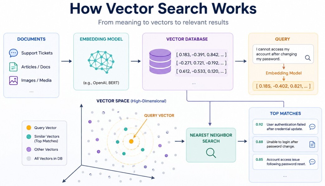
I cannot access my account after changing my password.
User authentication failed after credential update.
A vector database transforms the problem of "finding documents containing similar words" into "finding vectors that are located close to each other" in a mathematical space.
Why SQL Fails Semantic Retrieval?
Traditional relational databases were created for structured data. They are extremely powerful when the question is deterministic.For example:
SELECT *
FROM tickets
WHERE status = 'OPEN'
AND priority = 'HIGH';
It does not ask: "Which records contain this exact value?". It asks: "Which records express a similar meaning?"
A SQL index does not understand that:
Reset my password
Recover forgotten login credentials
This limitation exists because traditional indexes organize information based on exact values, while semantic systems organize information based on relationships between meanings.
Full-text search engines improved this using inverted indexes, stemming, and ranking algorithms like BM25, but they still fundamentally depend on lexical similarity.
Inverted IndexesModern AI applications require semantic similarity, where two completely different sentences can still be considered close.
- Stores a mapping of unique words to the documents containing them.
- Acts like a textbook index for lightning-fast lookups.
- Eliminates the need to scan entire databases sequentially.
Stemming
- Reduces words to their base form by stripping suffixes.
- Groups variations like "running" and "runs" into "run".
- Ensures queries match documents using different word forms.
BM25 Ranking
- Scores document relevance using word frequency and rarity.
- Penalizes overly long documents through length normalization.
- Prevents repetitive words from unfairly inflating the score.
Semantic similarity is a metric that measures how closely two pieces of text relate in meaning, regardless of whether they share the same words. It evaluates the underlying context and conceptual resemblance rather than relying on exact, literal word matches.
What Is Vector Search?
Vector search is the process of finding vectors that are mathematically closest to a given query vector. When documents enter a semantic search system, each document passes through an embedding model.Document → Embedding Model → Vector → Vector DatabaseAn embedding model is a type of machine learning model that converts complex, unstructured data (like words, sentences, or images) into arrays of numbers called vectors.The database stores this vector representation. A simplified stored object looks like:
Depending on the data you need to analyze, you will use different embedding models:
1. Text Embeddings: Models designed to process language. Popular examples include BERT, Word2Vec, and models from providers like Cohere or OpenAI.
2. Image Embeddings: Models that convert images into vectors so that visually similar photos can be found or clustered together.
3. Audio Embeddings: Models that turn raw speech or music into vectors, powering speech recognition.
{
    "id": "ticket-10291",

    "vector": [
        0.183,
        -0.391,
        0.842
    ],

    "metadata": {
        "category": "authentication",
        "customer": "enterprise"
    }
}
User Query → Embedding Model → Query Vector → Nearest Neighbor Search → Relevant DocumentsUnderstanding Similarity Measurement
Once everything becomes vectors, the most important question becomes: How do we calculate whether two vectors are similar?There are multiple similarity metrics, and choosing the right one impacts retrieval accuracy. The most commonly used techniques are Cosine Similarity, Euclidean Distance, and Dot Product Similarity.
Cosine Similarity
Cosine similarity measures the angle between two vectors. The important idea is that it cares about direction, not length. Two sentences may produce vectors with different magnitudes, but if they point in the same direction, they represent similar meaning.The mathematical formula is:
Cosine Similarity = (A · B) / (||A|| × ||B||)
import numpy as np
from sentence_transformers import SentenceTransformer

# 1. Load a lightweight, high-performance semantic model
model = SentenceTransformer("all-MiniLM-L6-v2")

# 2. Define the sentences
sentence_A = "Forgot my password"
sentence_B = "Cannot login because credentials are lost"

# 3. Generate the embeddings (vectors)
embedding_A = model.encode(sentence_A)
embedding_B = model.encode(sentence_B)

# 4. Compute cosine similarity: (A • B) / (||A|| * ||B||)
def cosine_similarity(v1, v2):
    dot_product = np.dot(v1, v2)
    norm_v1 = np.linalg.norm(v1)
    norm_v2 = np.linalg.norm(v2)
    return dot_product / (norm_v1 * norm_v2)

score = cosine_similarity(embedding_A, embedding_B)

print(f"Sentence A: {sentence_A}")
print(f"Sentence B: {sentence_B}\n")
print(f"Cosine Score: {score:.2f}")
Sentence A: Forgot my password
Sentence B: Cannot login because credentials are lost

Cosine Score: 0.61
Euclidean Distance
Euclidean distance measures the actual physical distance between two vectors. It answers: "How far apart are these two points?". Because it factors in vector magnitude (length), longer texts can yield a larger distance even if they mean the same thing.The formula is:
Distance = sqrt((x1 - x2)^2 + (y1 - y2)^2)import numpy as np
from sentence_transformers import SentenceTransformer
# 1. Load the model
model = SentenceTransformer("all-MiniLM-L6-v2")
# 2. Define the sentences
sentence_A = "Forgot my password"
sentence_B = "Cannot login because credentials are lost"
# 3. Generate embeddings
embedding_A = model.encode(sentence_A)
embedding_B = model.encode(sentence_B)
# 4. Compute Euclidean Distance: sqrt(sum((A - B)^2))
def euclidean_distance(v1, v2):
return np.linalg.norm(v1 - v2)
distance = euclidean_distance(embedding_A, embedding_B)
print(f"Sentence A: {sentence_A}")
print(f"Sentence B: {sentence_B}\n")
print(f"Euclidean Distance: {distance:.2f}") # Lower means closer/more similar
Sentence A: Forgot my password
Sentence B: Cannot login because credentials are lost

Euclidean Distance: 0.89
Cosine Similarity: (1.0) is a perfect match (higher is better).
Euclidean Distance: (0.0) is a perfect match (lower is better).
Dot Product Similarity
Dot product similarity multiplies corresponding vector dimensions and adds the results together.A = [1,2,3]
B = [4,5,6]
Dot Product: (1×4) + (2×5) + (3×6) = 32
A larger dot product generally means stronger similarity. Dot product measures both the angle and the magnitude (length) of two vectors. If you normalize your embeddings first to a length of 1, the dot product will give you the exact same ranking as cosine similarity.
import numpy as np
from sentence_transformers import SentenceTransformer

# 1. Load the model
model = SentenceTransformer("all-MiniLM-L6-v2")

# 2. Define the sentences
sentence_A = "Forgot my password"
sentence_B = "Cannot login because credentials are lost"

# 3. Generate embeddings
embedding_A = model.encode(sentence_A)
embedding_B = model.encode(sentence_B)

# 4. Compute Dot Product: sum(A * B)
def dot_product_similarity(v1, v2):
    return np.dot(v1, v2)

score = dot_product_similarity(embedding_A, embedding_B)

print(f"Sentence A: {sentence_A}")
print(f"Sentence B: {sentence_B}\n")
print(f"Dot Product Score: {score:.2f}")  # Higher means more similar
Sentence A: Forgot my password
Sentence B: Cannot login because credentials are lost

Dot Product Score: 0.61
A normalized vector (or unit vector) is a vector that has been scaled so that its total mathematical length (magnitude) equals exactly 1.0, while its direction remains completely unchanged. In machine learning and NLP, normalization strips away the "noise" of text length.Many deep-learning recommendation systems use dot product because magnitude can represent confidence, popularity, or strength of a relationship.
To normalize a vector, you divide each coordinate in the vector by the vector's total length (known as the L2 norm or Euclidean length).
Normalized Vector = V / ||V||
If you normalize your embeddings before saving them to a vector database, you unlock two massive engineering advantages:
1. Math Shortcut: Cosine Similarity and Dot Product become the exact same math operation. Because the lengths are already (1.0), the denominator in the cosine formula disappears.
2. Speed Boost: You can replace the slow Cosine Similarity calculation with a raw Dot Product. This removes expensive square root calculations, saving massive CPU/GPU cycles during large-scale vector searches.
Here is how you manually normalize vectors using numpy and verify their lengths:import numpy as np # A raw embedding vector from a model (magnitudes vary) raw_vector = np.array([3.0, 4.0, 0.0]) # 1. Calculate the current length (L2 Norm) -> sqrt(3^2 + 4^2) = 5.0 current_length = np.linalg.norm(raw_vector) # 2. Normalize by dividing the vector by its length normalized_vector = raw_vector / current_length # Result: [0.6, 0.8, 0.0] # 3. Verify the new length is exactly 1.0 new_length = np.linalg.norm(normalized_vector) print(f"Original Vector: {raw_vector}") print(f"Original Length: {current_length}") print(f"Normalized Vector: {normalized_vector}") print(f"Verified Length: {new_length:.1f}")Original Vector: [3. 4. 0.] Original Length: 5.0 Normalized Vector: [0.6 0.8 0. ] Verified Length: 1.0
Why Brute Force Search Becomes Impossible?
The simplest implementation of vector search is comparing the query vector against every stored vector.for document in documents:
similarity = cosine_similarity(
query_vector,
document.vector
)
results.append(similarity)
However, imagine a production system:
- 50 million support tickets
- 1536 dimensions per vector
- Thousands of searches every second
Every query would require billions of mathematical operations. Even with powerful hardware, latency becomes unacceptable. Real search systems need responses in milliseconds. This scaling challenge introduced Approximate Nearest Neighbor Search.
Approximate Nearest Neighbor Search (ANN)
ANN solves the scalability problem by changing the goal. Instead of asking: "Find the absolute closest vector by checking everything." It asks: "Find a vector that is almost certainly among the closest results but do it extremely fast."This small accuracy tradeoff produces massive performance improvements. Production search systems prefer returning a 99% accurate result in 20 milliseconds instead of a perfect result in several seconds.
Popular ANN approaches include HNSW, IVF, and Product Quantization.
Hierarchical Navigable Small World (HNSW)
HNSW optimizes vector search by replacing a brute-force O(N) linear scan with an O(log N) graph traversal. Instead of calculating distances against every vector, it structures embeddings into a multi-layer graph where proximate vectors are linked as neighbors.Imagine a city with millions of houses. If you want to find one house, you do not check every house one by one. You first use highways, then main roads, then local streets. HNSW follows a similar strategy.
HNSW replicates a skip-list data structure across geometric space, isolating routing into hierarchical layers:
The structure looks conceptually like:
Layer 3 (Express):     A ----------------------- Z  (Massive spatial jumps)
Layer 2 (Highway):     A -------- M ------------ Z  (Regional routing)
Layer 1 (Main Road):   A -- B -- C -- D -- E --- Z  (Local clusters)
Layer 0 (Dense Graph): [All vectors connected locally]
2. It aggressively traverses paths toward neighbors closest to the query vector, skipping irrelevant clusters entirely.
3. When a local minimum is reached on a layer, the algorithm drops to the exact same spatial coordinate in the layer below.
4. It repeats this process down to Layer 0, executing a highly focused, localized neighborhood search for exact nearest neighbors.
It bypasses millions of expensive high-dimensional distance array operations. Data links favor local memory layouts, minimizing CPU cache misses during traversal loops. This predictable latency profile makes HNSW the default index driver for Qdrant, Weaviate, and Elasticsearch.
HNSW Production Tuning
HNSW performance depends heavily on configuration. Two important parameters engineers usually tune are M and ef_search.The parameter M controls how many connections each vector maintains with neighboring vectors. Higher values create a richer graph. This improves search quality because the algorithm has more paths available, but it increases memory usage.
Higher M → Better accuracy → More RAM usage
Lower M → Less memory → Possible accuracy reduction
The parameter ef_search controls how many candidate vectors are explored during searching. A larger value improves recall because the algorithm investigates more possibilities.
However, more exploration means higher latency.
High ef_search → Better retrieval quality → Slower response
Low ef_search → Faster response → Lower accuracy
Production vector search is always a balance between: Accuracy vs Latency vs Memory Cost
Inverted File Index (IVF)
Another important ANN technique is Inverted File Index (IVF). The idea behind IVF is clustering. Instead of storing millions of vectors together, IVF divides the vector space into different regions.During indexing, similar vectors are grouped into clusters.
Vector Space

Cluster A → password login authentication
Cluster B → docker kubernetes deployment
Cluster C → payment invoice billing
This significantly reduces computation. However, there is a tradeoff. If the wrong cluster is selected, some relevant vectors may never be checked. Therefore IVF systems tune how many clusters should be searched for each query.
Product Quantization (PQ)
At billion-vector scale, another challenge appears. Memory consumption becomes enormous. The storage requirement can easily reach terabytes. Keeping everything in memory becomes extremely expensive.Product Quantization (PQ) solves this by compressing vectors. Instead of storing full precision vectors, PQ stores approximate representations. For example:
Original Vector: [0.18392, -0.83911, 0.77421]
Compressed Representation: [12, 81, 45]
Qdrant Vector Database
Qdrant is an open-source, production-ready vector similarity search engine and vector database written in Rust. It is specifically engineered to store, manage, and search high-dimensional vector embeddings along with additional JSON payloads (metadata).It delivers ultra-fast, low-latency performance at scale, making it a foundation for generative AI, semantic search, and recommendation pipelines. A simple example of storing vectors using Qdrant:
from qdrant_client import QdrantClient
from qdrant_client.models import PointStruct

client = QdrantClient(
    host="localhost",
    port=6333
)

client.upsert(
    collection_name="tickets",
    points=[
        PointStruct(
            id=1,
            vector=[
                0.12,
                0.87,
                0.45
            ],
            payload={
                "text":
                "Password reset failure"
            }
        )
    ]
)
results = client.search(
    collection_name="tickets",
    query_vector=[
        0.11,
        0.84,
        0.40
    ],
    limit=5
)

for result in results:
    print(result.payload)
Elasticsearch Vector Database
Elasticsearch is a distributed search and analytics engine that functions as a robust vector database, allowing you to store, index, and search high-dimensional vector embeddings.By combining traditional lexical search with modern vector search, it provides a unified platform for building AI-driven applications like semantic search and Retrieval-Augmented Generation (RAG).
A document can store embeddings using a dense_vector field.
{
  "mappings": {
    "properties": {
      "content_vector": {
        "type": "dense_vector",
        "dims": 1536,
        "index": true,
        "similarity": "cosine"
      }
    }
  }
}
{
  "knn": {
    "field": "content_vector",
    "query_vector": [
        0.12,
        0.88,
        0.44
    ],
    "k": 10
  }
}
Choosing Between Pinecone, Weaviate, Qdrant, and Elasticsearch
Different vector databases optimize for different production requirements.| Vector Database | Description | Best Suitable For |
|---|---|---|
| Pinecone | Fully managed vector database focused on simplicity, scalability, and large-scale cloud deployments. | Managed cloud-based AI applications and enterprise-scale RAG systems. |
| Qdrant | Provides excellent performance, powerful metadata filtering, and efficient vector search capabilities. | Self-hosted production environments requiring high performance and control. |
| Weaviate | Combines vector search with knowledge-graph-style capabilities and built-in AI integrations. | AI-native applications requiring semantic search with rich data relationships. |
| Elasticsearch | Provides hybrid keyword and vector search capabilities without introducing a separate search system. | Organizations already using Elasticsearch and needing semantic search. |
Conclusion
Vector databases are the retrieval engines behind modern AI applications. Embeddings transform meaning into mathematical space, while vector databases make searching that space possible at massive scale.Similarity metrics such as Cosine Similarity, Euclidean Distance, and Dot Product define how closeness is measured.
Algorithms such as HNSW, IVF, and Product Quantization solve the challenge of searching billions of vectors with millisecond latency.
In the next article, we will move beyond retrieval and explore how production AI systems improve search accuracy using rerankers, hybrid search, query rewriting, and retrieval evaluation metrics.