PostgreSQL is one of the best choices for such workloads because it is ACID-compliant, mature, and highly reliable. The 17.x series also introduces meaningful improvements in query planning and logical replication.
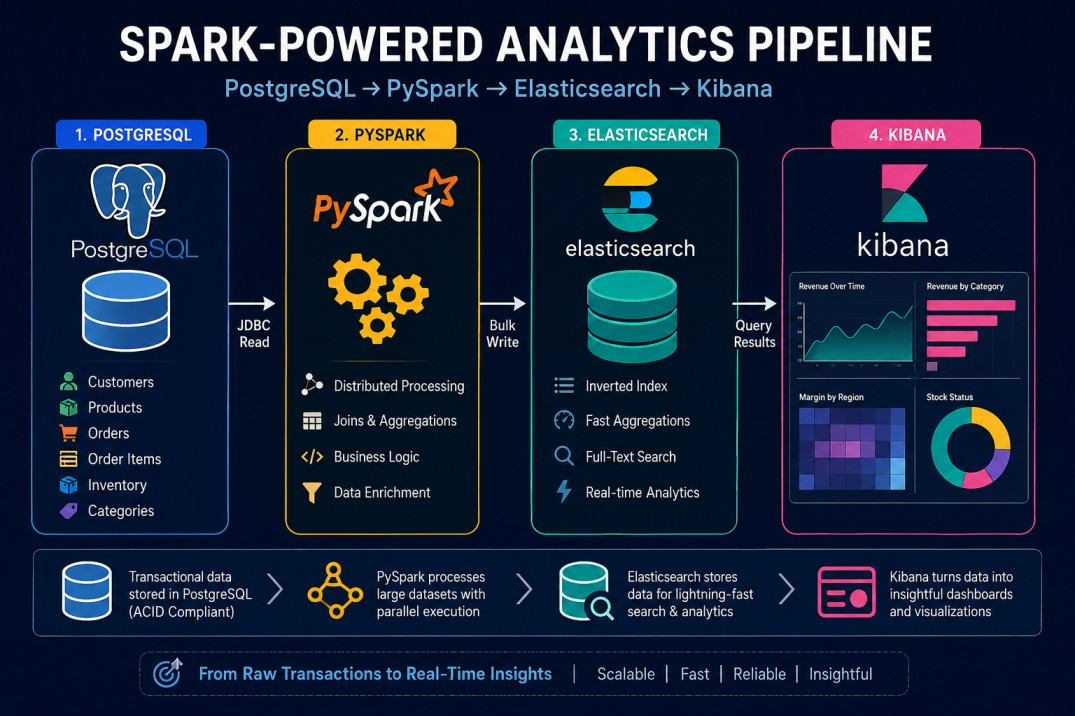
An OLTP (Online Transaction Processing) database is a system designed to manage day-to-day, real-time operations and transactions. It prioritizes high-speed, concurrent read/write operations (like inserting, updating, or deleting small amounts of data) and strictly maintains data integrity.Apache Spark bridges the gap. Spark reads the relational data over JDBC, performs large-scale joins and aggregations across its distributed executor pool, and produces enriched, denormalised documents.
Those documents then flow into Elasticsearch, where they are stored in inverted indices optimised for sub-second aggregation queries. Kibana sits on top, turning those indices into live dashboards your operations and business teams can actually use.
| Step | Component | Version |
|---|---|---|
| 1 | PostgreSQL | 17.9 |
| 2 | PySpark | 4.1.x |
| 3 | Elasticsearch | 9.4.x |
| 4 | Kibana | 9.4.x |
Next we write PySpark jobs that read multiple tables, join them, and compute sales analytics. Finally we push the results to Elasticsearch and build a Kibana dashboard. Every piece of infrastructure configuration, SQL, and Python code is shown in full.
Infrastructure Setup with Docker Compose
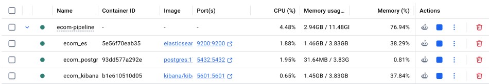
The simplest way to run all four components locally is Docker Compose. The file below pins every image to the exact versions required by this article. Notice that Elasticsearch and Kibana must share the same minor version - mismatches cause the Kibana startup to fail with a compatibility error.We also disable Elasticsearch's built-in security for local development; you would never do this in production.
docker-compose.yml
version: "3.9"

services:

  postgres:
    image: postgres:17.9
    container_name: ecom_postgres
    environment:
      POSTGRES_USER: ecom
      POSTGRES_PASSWORD: ecom_secret
      POSTGRES_DB: ecomdb
    ports:
      - "5433:5432"
    volumes:
      - pgdata:/var/lib/postgresql/data
      - ./sql/init.sql:/docker-entrypoint-initdb.d/init.sql
    healthcheck:
      test: ["CMD-SHELL", "pg_isready -U ecom -d ecomdb"]
      interval: 10s
      timeout: 5s
      retries: 5

  elasticsearch:
    image: docker.elastic.co/elasticsearch/elasticsearch:9.4.0
    container_name: ecom_es
    environment:
      - discovery.type=single-node
      - xpack.security.enabled=false
      - xpack.security.http.ssl.enabled=false
      - ES_JAVA_OPTS=-Xms1g -Xmx1g
    ports:
      - "9200:9200"
    volumes:
      - esdata:/usr/share/elasticsearch/data
    healthcheck:
      test: ["CMD-SHELL", "curl -s http://localhost:9200/_cluster/health | grep -q '\"status\":\"green\"\\|\"status\":\"yellow\"'"]
      interval: 15s
      timeout: 10s
      retries: 10

  kibana:
    image: docker.elastic.co/kibana/kibana:9.4.0
    container_name: ecom_kibana
    environment:
      - ELASTICSEARCH_HOSTS=http://elasticsearch:9200
    ports:
      - "5601:5601"
    depends_on:
      elasticsearch:
        condition: service_healthy

volumes:
  pgdata:
  esdata:
docker compose up -d. PostgreSQL will automatically run the init.sql file on first boot, we will create that file in the next section. Give Elasticsearch about 30 seconds to reach yellow health status before proceeding; you can monitor it with docker compose logs -f elasticsearch.
Create a Python virtual environment and install dependencies:
python3.13 -m venv .venv
source .venv/bin/activate

# PySpark 4.1.x ships Spark 4.1 under the hood
pip install pyspark==4.1.0
pip install psycopg2-binary==2.9.10
pip install elasticsearch==9.0.0
pip install python-dateutil faker
mkdir -p jars
curl -L -o jars/postgresql-42.7.4.jar https://jdbc.postgresql.org/download/postgresql-42.7.4.jar
PostgreSQL Schema and Seed Data
Good analytical work starts with a realistic schema. Our e-commerce domain has six core tables: customers, products, categories, orders, order_items, and inventory.The relationships are intentionally normalised, that tension between normalisation and analytical read performance is exactly why Spark and Elasticsearch exist in this stack.
| Table | Key Columns | Purpose |
|---|---|---|
| categories | category_id, name, parent_id | Hierarchical product taxonomy |
| products | product_id, category_id, sku, name, price, cost | Product catalogue with margin data |
| customers | customer_id, email, region, tier | Customer master with segmentation |
| orders | order_id, customer_id, status, order_date, shipped_date | Order header, state machine |
| order_items | item_id, order_id, product_id, qty, unit_price | Line items; the fact table |
| inventory | product_id, warehouse, qty_on_hand, reorder_point | Current stock levels per warehouse |
sql/init.sql. PostgreSQL will execute this automatically when the container first boots. The schema uses identity columns (the modern Postgres alternative to sequences), proper foreign key constraints, and a check constraint to enforce the order state machine.
The seed data below gives us 1,000 orders spread across 200 customers, 80 products in 12 categories, and three warehouses,-enough to generate visually interesting Kibana charts.
init.sql
-- ──────────────────────────────────────────────
-- E-Commerce Schema for Spark / ES pipeline demo
-- PostgreSQL 17.9
-- ──────────────────────────────────────────────

SET client_min_messages = warning;

-- ── CATEGORIES ──────────────────────────────────
CREATE TABLE categories (
    category_id   INT  GENERATED ALWAYS AS IDENTITY PRIMARY KEY,
    name          TEXT NOT NULL UNIQUE,
    parent_id     INT  REFERENCES categories(category_id)
);

INSERT INTO categories (name, parent_id) VALUES
    ('Electronics',       NULL),
    ('Clothing',          NULL),
    ('Home & Garden',     NULL),
    ('Sports',            NULL),
    ('Books',             NULL),
    ('Smartphones',       1),
    ('Laptops',           1),
    ('Audio',             1),
    ('Mens Apparel',      2),
    ('Womens Apparel',    2),
    ('Kitchen',           3),
    ('Outdoor Sports',    4);

-- ── PRODUCTS ────────────────────────────────────
CREATE TABLE products (
    product_id    INT     GENERATED ALWAYS AS IDENTITY PRIMARY KEY,
    category_id   INT     NOT NULL REFERENCES categories(category_id),
    sku           TEXT    NOT NULL UNIQUE,
    name          TEXT    NOT NULL,
    price         NUMERIC(10,2) NOT NULL CHECK (price > 0),
    cost          NUMERIC(10,2) NOT NULL CHECK (cost > 0),
    is_active     BOOLEAN NOT NULL DEFAULT TRUE,
    created_at    TIMESTAMPTZ NOT NULL DEFAULT now()
);

INSERT INTO products (category_id, sku, name, price, cost) VALUES
    -- Smartphones (cat 6)
    (6,  'SP-001', 'ProPhone 15 Ultra',      1099.00,  620.00),
    (6,  'SP-002', 'ProPhone 15 Standard',    799.00,  420.00),
    (6,  'SP-003', 'BudgetPhone Z1',          299.00,  140.00),
    (6,  'SP-004', 'MidPhone X5',             549.00,  280.00),
    -- Laptops (cat 7)
    (7,  'LP-001', 'DevBook Pro 16',         1899.00, 1050.00),
    (7,  'LP-002', 'DevBook Air 14',         1199.00,  620.00),
    (7,  'LP-003', 'OfficeBook 15',           699.00,  350.00),
    (7,  'LP-004', 'GamingBook RTX',         2299.00, 1380.00),
    -- Audio (cat 8)
    (8,  'AU-001', 'SoundBar X900',           349.00,  160.00),
    (8,  'AU-002', 'NoiseCancelPro Headset',  329.00,  145.00),
    (8,  'AU-003', 'TrueWireless Buds',       129.00,   52.00),
    (8,  'AU-004', 'Studio Monitor Pair',     599.00,  290.00),
    -- Mens Apparel (cat 9)
    (9,  'MA-001', 'Classic Crew Tee',         29.00,    8.00),
    (9,  'MA-002', 'Slim Fit Chinos',          79.00,   22.00),
    (9,  'MA-003', 'Performance Polo',         59.00,   16.00),
    (9,  'MA-004', 'Winter Parka',            199.00,   78.00),
    -- Womens Apparel (cat 10)
    (10, 'WA-001', 'Floral Sundress',          89.00,   28.00),
    (10, 'WA-002', 'Yoga Leggings',            65.00,   21.00),
    (10, 'WA-003', 'Cashmere Pullover',       179.00,   72.00),
    (10, 'WA-004', 'Rain Jacket',             149.00,   58.00),
    -- Kitchen (cat 11)
    (11, 'KT-001', 'Espresso Machine Pro',    449.00,  195.00),
    (11, 'KT-002', 'Cast Iron Skillet Set',    89.00,   32.00),
    (11, 'KT-003', 'High-Speed Blender',      179.00,   72.00),
    (11, 'KT-004', 'Digital Air Fryer 6L',    129.00,   49.00),
    -- Outdoor Sports (cat 12)
    (12, 'OS-001', 'Trail Running Shoes',     159.00,   61.00),
    (12, 'OS-002', 'Carbon Fibre Tent 2P',    399.00,  165.00),
    (12, 'OS-003', 'Trekking Poles Pair',      79.00,   28.00),
    (12, 'OS-004', 'Hydration Backpack 20L',  119.00,   44.00),
    -- Books (cat 5)
    (5,  'BK-001', 'Data Engineering Handbook', 49.00, 12.00),
    (5,  'BK-002', 'Clean Architecture',        39.00,  9.00);

-- ── CUSTOMERS ───────────────────────────────────
CREATE TABLE customers (
    customer_id   INT  GENERATED ALWAYS AS IDENTITY PRIMARY KEY,
    email         TEXT NOT NULL UNIQUE,
    first_name    TEXT NOT NULL,
    last_name     TEXT NOT NULL,
    region        TEXT NOT NULL CHECK (region IN ('NORTH','SOUTH','EAST','WEST','CENTRAL')),
    tier          TEXT NOT NULL CHECK (tier IN ('BRONZE','SILVER','GOLD','PLATINUM')) DEFAULT 'BRONZE',
    registered_at TIMESTAMPTZ NOT NULL DEFAULT now()
);

-- Seed 200 customers across regions and tiers
INSERT INTO customers (email, first_name, last_name, region, tier)
SELECT
    'user' || n || '@example.com',
    (ARRAY['Alice','Bob','Carol','David','Eva','Frank','Grace','Hiro','Iris','Jake'])[1 + (n % 10)],
    (ARRAY['Smith','Jones','Brown','Williams','Taylor','Davies','Evans','Wilson','Thomas','Roberts'])[1 + ((n * 3) % 10)],
    (ARRAY['NORTH','SOUTH','EAST','WEST','CENTRAL'])[1 + (n % 5)],
    (ARRAY['BRONZE','BRONZE','SILVER','SILVER','GOLD','PLATINUM'])[1 + (n % 6)]
FROM generate_series(1, 200) AS n;

-- ── ORDERS ──────────────────────────────────────
CREATE TABLE orders (
    order_id      INT  GENERATED ALWAYS AS IDENTITY PRIMARY KEY,
    customer_id   INT  NOT NULL REFERENCES customers(customer_id),
    status        TEXT NOT NULL CHECK (status IN ('PENDING','CONFIRMED','SHIPPED','DELIVERED','CANCELLED','RETURNED')),
    order_date    TIMESTAMPTZ NOT NULL,
    shipped_date  TIMESTAMPTZ,
    channel       TEXT NOT NULL CHECK (channel IN ('WEB','MOBILE','MARKETPLACE','RETAIL')),
    coupon_code   TEXT,
    discount_pct  NUMERIC(5,2) NOT NULL DEFAULT 0 CHECK (discount_pct >= 0 AND discount_pct <= 100)
);

-- Seed 1 000 orders spread across the last 365 days
INSERT INTO orders (customer_id, status, order_date, shipped_date, channel, discount_pct)
SELECT
    1 + (n % 200) AS customer_id,
    (ARRAY['PENDING','CONFIRMED','SHIPPED','DELIVERED','DELIVERED','DELIVERED','CANCELLED','RETURNED'])[1 + (n % 8)] AS status,
    now() - (random() * interval '365 days') AS order_date,
    CASE WHEN (n % 8) BETWEEN 2 AND 5
         THEN now() - (random() * interval '300 days')
         ELSE NULL
    END AS shipped_date,
    (ARRAY['WEB','WEB','MOBILE','MARKETPLACE','RETAIL'])[1 + (n % 5)] AS channel,
    (ARRAY[0,0,5,10,15,20])[1 + (n % 6)] AS discount_pct
FROM generate_series(1, 1000) AS n;

-- ── ORDER_ITEMS ──────────────────────────────────
CREATE TABLE order_items (
    item_id       INT  GENERATED ALWAYS AS IDENTITY PRIMARY KEY,
    order_id      INT  NOT NULL REFERENCES orders(order_id),
    product_id    INT  NOT NULL REFERENCES products(product_id),
    quantity      INT  NOT NULL CHECK (quantity > 0),
    unit_price    NUMERIC(10,2) NOT NULL CHECK (unit_price >= 0)
);

-- Seed 2-4 line items per order (≈3 000 rows total)
INSERT INTO order_items (order_id, product_id, quantity, unit_price)
SELECT
    o.order_id,
    1 + (row_number() OVER (PARTITION BY o.order_id ORDER BY random())::INT % 30) AS product_id,
    1 + (random() * 3)::INT AS quantity,
    p.price * (1 - o.discount_pct / 100) AS unit_price
FROM orders o
CROSS JOIN LATERAL (
    SELECT generate_series(1, 2 + (o.order_id % 3)) AS line_num
) lines
JOIN LATERAL (
    SELECT price FROM products
    ORDER BY random()
    LIMIT 1
) p ON TRUE;

-- ── INVENTORY ───────────────────────────────────
CREATE TABLE inventory (
    inventory_id   INT  GENERATED ALWAYS AS IDENTITY PRIMARY KEY,
    product_id     INT  NOT NULL REFERENCES products(product_id),
    warehouse      TEXT NOT NULL CHECK (warehouse IN ('WH-EAST','WH-WEST','WH-CENTRAL')),
    qty_on_hand    INT  NOT NULL CHECK (qty_on_hand >= 0),
    reorder_point  INT  NOT NULL CHECK (reorder_point >= 0),
    last_updated   TIMESTAMPTZ NOT NULL DEFAULT now(),
    UNIQUE (product_id, warehouse)
);

-- One row per product per warehouse
INSERT INTO inventory (product_id, warehouse, qty_on_hand, reorder_point)
SELECT
    p.product_id,
    w.warehouse,
    (random() * 400 + 10)::INT AS qty_on_hand,
    (random() * 50 + 5)::INT  AS reorder_point
FROM products p
CROSS JOIN (
    VALUES ('WH-EAST'), ('WH-WEST'), ('WH-CENTRAL')
) AS w(warehouse);

-- ── INDEXES FOR JDBC PARTITION QUERIES ──────────
CREATE INDEX ON orders (order_date);
CREATE INDEX ON orders (customer_id);
CREATE INDEX ON order_items (order_id);
CREATE INDEX ON order_items (product_id);
CREATE INDEX ON inventory (product_id);

-- ── VERIFY ──────────────────────────────────────
SELECT 'categories'  AS tbl, count(*) FROM categories
UNION ALL SELECT 'products',   count(*) FROM products
UNION ALL SELECT 'customers',  count(*) FROM customers
UNION ALL SELECT 'orders',     count(*) FROM orders
UNION ALL SELECT 'order_items',count(*) FROM order_items
UNION ALL SELECT 'inventory',  count(*) FROM inventory;
PySpark Environment and SparkSession
Every PySpark application begins with a SparkSession, the unified entry point introduced in Spark 2.0 that replaced the olderSparkContext and SQLContext combination. When running locally, the session spawns a single JVM process with multiple threads simulating distributed execution.
The two JDBC JARs we downloaded must be listed in the
spark.jars configuration at session creation time; they cannot be added after the JVM has started.
Create a file called
spark_session.py that we will import from every job. This keeps configuration in one place and avoids repetition:
spark_session.py
"""
Shared SparkSession factory for the ecom pipeline.
Compatible with PySpark 4.1.x / Python 3.13.
"""
import os
from pyspark.sql import SparkSession

PG_URL  = "jdbc:postgresql://localhost:5433/ecomdb"
PG_PROPS = {
    "user":     "ecom",
    "password": "ecom_secret",
    "driver":   "org.postgresql.Driver",
}

ES_HOST = "localhost"
ES_PORT = "9200"

# Only JDBC JAR — ES writes use elasticsearch-py via foreachPartition
_HERE    = os.path.dirname(os.path.abspath(__file__))
JDBC_JAR = os.path.join(_HERE, "jars", "postgresql-42.7.4.jar")


def get_spark(app_name: str = "EcomPipeline") -> SparkSession:
    return (
        SparkSession.builder
        .appName(app_name)
        .master("local[*]")
        .config("spark.jars", JDBC_JAR)
        .config("spark.serializer", "org.apache.spark.serializer.KryoSerializer")
        .config("spark.sql.shuffle.partitions", "8")
        .config("spark.sql.adaptive.enabled", "true")
        .getOrCreate()
    )
Reading from PostgreSQL with PySpark
Reading a table over JDBC is a one-liner in PySpark, but doing it naively will send a single sequential scan from a single Spark executor. For small tables this is fine, but fororder_items with its millions of rows you want JDBC partitioning, Spark issues multiple parallel queries, each fetching a different range of the partition column, and distributes the work across its executor pool.
The key parameters are
partitionColumn (must be a numeric or date column), lowerBound, upperBound, and numPartitions.
Create
read_postgres.py. We define helper functions for small dimension tables (single read) and large fact tables (partitioned read), then expose a single function that returns all six tables as a dictionary of DataFrames:
read_postgres.py
"""
Read all ecom tables from PostgreSQL into PySpark DataFrames.
"""
from pyspark.sql import SparkSession, DataFrame
from spark_session import PG_URL, PG_PROPS


def _read_table(spark: SparkSession, table: str) -> DataFrame:
    """Simple single-partition read – for small dimension tables."""
    return (
        spark.read
        .format("jdbc")
        .option("url", PG_URL)
        .option("dbtable", table)
        .options(**PG_PROPS)
        .load()
    )


def _read_partitioned(
    spark: SparkSession,
    table: str,
    partition_col: str,
    lower: int,
    upper: int,
    num_partitions: int = 8,
) -> DataFrame:
    """
    Partitioned JDBC read.  Spark issues `num_partitions` parallel queries
    each covering a range of `partition_col` values.
    """
    return (
        spark.read
        .format("jdbc")
        .option("url", PG_URL)
        .option("dbtable", table)
        .option("partitionColumn", partition_col)
        .option("lowerBound",      str(lower))
        .option("upperBound",      str(upper))
        .option("numPartitions",   str(num_partitions))
        .options(**PG_PROPS)
        .load()
    )


def load_all_tables(spark: SparkSession) -> dict[str, DataFrame]:
    """
    Return a dict mapping table name → DataFrame for all six tables.
    Dimension tables use a single read; fact tables use partitioning.
    """
    print("[read_postgres] Loading dimension tables …")
    categories = _read_table(spark, "categories")
    products   = _read_table(spark, "products")
    customers  = _read_table(spark, "customers")
    inventory  = _read_table(spark, "inventory")

    print("[read_postgres] Loading fact tables with partitioning …")
    orders = _read_partitioned(
        spark, "orders",
        partition_col   = "order_id",
        lower           = 1,
        upper           = 1100,   # slightly above max for safety
        num_partitions  = 8,
    )

    order_items = _read_partitioned(
        spark, "order_items",
        partition_col   = "item_id",
        lower           = 1,
        upper           = 4000,
        num_partitions  = 8,
    )

    tables = {
        "categories":  categories,
        "products":    products,
        "customers":   customers,
        "inventory":   inventory,
        "orders":      orders,
        "order_items": order_items,
    }

    for name, df in tables.items():
        print(f"  {name:15s}  {df.count():>6,} rows  |  schema: {df.dtypes}")

    return tables


if __name__ == "__main__":
    from spark_session import get_spark
    spark = get_spark("ReadPostgres")
    tables = load_all_tables(spark)
    for name, df in tables.items():
        print(f"\n── {name} ──")
        df.show(5, truncate=False)
    spark.stop()
python read_postgres.py. You should see row counts and five sample rows from each table printed to the console.
.
.
.
[read_postgres] Loading dimension tables …
[read_postgres] Loading fact tables with partitioning …
  categories           12 rows  |  schema: [('category_id', 'int'), ('name', 'string'), ('parent_id', 'int')]
  products             30 rows  |  schema: [('product_id', 'int'), ('category_id', 'int'), ('sku', 'string'), ('name', 'string'), ('price', 'decimal(10,2)'), ('cost', 'decimal(10,2)'), ('is_active', 'boolean'), ('created_at', 'timestamp')]
  customers           200 rows  |  schema: [('customer_id', 'int'), ('email', 'string'), ('first_name', 'string'), ('last_name', 'string'), ('region', 'string'), ('tier', 'string'), ('registered_at', 'timestamp')]
  inventory            90 rows  |  schema: [('inventory_id', 'int'), ('product_id', 'int'), ('warehouse', 'string'), ('qty_on_hand', 'int'), ('reorder_point', 'int'), ('last_updated', 'timestamp')]
  orders            1,000 rows  |  schema: [('order_id', 'int'), ('customer_id', 'int'), ('status', 'string'), ('order_date', 'timestamp'), ('shipped_date', 'timestamp'), ('channel', 'string'), ('coupon_code', 'string'), ('discount_pct', 'decimal(5,2)')]
  order_items       3,000 rows  |  schema: [('item_id', 'int'), ('order_id', 'int'), ('product_id', 'int'), ('quantity', 'int'), ('unit_price', 'decimal(10,2)')]

── categories ──
+-----------+-------------+---------+
|category_id|name         |parent_id|
+-----------+-------------+---------+
|1          |Electronics  |NULL     |
|2          |Clothing     |NULL     |
|3          |Home & Garden|NULL     |
|4          |Sports       |NULL     |
|5          |Books        |NULL     |
+-----------+-------------+---------+
only showing top 5 rows

── products ──
+----------+-----------+------+--------------------+-------+-------+---------+--------------------------+
|product_id|category_id|sku   |name                |price  |cost   |is_active|created_at                |
+----------+-----------+------+--------------------+-------+-------+---------+--------------------------+
|1         |6          |SP-001|ProPhone 15 Ultra   |1099.00|620.00 |true     |2026-05-28 12:49:53.132774|
|2         |6          |SP-002|ProPhone 15 Standard|799.00 |420.00 |true     |2026-05-28 12:49:53.132774|
|3         |6          |SP-003|BudgetPhone Z1      |299.00 |140.00 |true     |2026-05-28 12:49:53.132774|
|4         |6          |SP-004|MidPhone X5         |549.00 |280.00 |true     |2026-05-28 12:49:53.132774|
|5         |7          |LP-001|DevBook Pro 16      |1899.00|1050.00|true     |2026-05-28 12:49:53.132774|
+----------+-----------+------+--------------------+-------+-------+---------+--------------------------+
only showing top 5 rows

── customers ──
+-----------+-----------------+----------+---------+-------+--------+--------------------------+
|customer_id|email            |first_name|last_name|region |tier    |registered_at             |
+-----------+-----------------+----------+---------+-------+--------+--------------------------+
|1          |user1@example.com|Bob       |Williams |SOUTH  |BRONZE  |2026-05-28 12:49:53.134217|
|2          |user2@example.com|Carol     |Evans    |EAST   |SILVER  |2026-05-28 12:49:53.134217|
|3          |user3@example.com|David     |Roberts  |WEST   |SILVER  |2026-05-28 12:49:53.134217|
|4          |user4@example.com|Eva       |Brown    |CENTRAL|GOLD    |2026-05-28 12:49:53.134217|
|5          |user5@example.com|Frank     |Davies   |NORTH  |PLATINUM|2026-05-28 12:49:53.134217|
+-----------+-----------------+----------+---------+-------+--------+--------------------------+
only showing top 5 rows

── inventory ──
+------------+----------+----------+-----------+-------------+-------------------------+
|inventory_id|product_id|warehouse |qty_on_hand|reorder_point|last_updated             |
+------------+----------+----------+-----------+-------------+-------------------------+
|1           |1         |WH-EAST   |69         |41           |2026-05-28 12:49:53.16403|
|2           |1         |WH-WEST   |370        |17           |2026-05-28 12:49:53.16403|
|3           |1         |WH-CENTRAL|299        |15           |2026-05-28 12:49:53.16403|
|4           |2         |WH-EAST   |212        |11           |2026-05-28 12:49:53.16403|
|5           |2         |WH-WEST   |79         |25           |2026-05-28 12:49:53.16403|
+------------+----------+----------+-----------+-------------+-------------------------+
only showing top 5 rows

── orders ──
+--------+-----------+---------+--------------------------+--------------------------+-----------+-----------+------------+
|order_id|customer_id|status   |order_date                |shipped_date              |channel    |coupon_code|discount_pct|
+--------+-----------+---------+--------------------------+--------------------------+-----------+-----------+------------+
|1       |2          |CONFIRMED|2026-04-21 01:16:05.168359|NULL                      |WEB        |NULL       |0.00        |
|2       |3          |SHIPPED  |2025-07-21 07:14:00.321576|2026-01-21 10:47:59.338759|MOBILE     |NULL       |5.00        |
|3       |4          |DELIVERED|2025-10-24 12:29:54.326842|2025-10-30 20:51:21.334158|MARKETPLACE|NULL       |10.00       |
|4       |5          |DELIVERED|2025-08-30 08:20:04.184441|2025-09-05 20:02:43.622241|RETAIL     |NULL       |15.00       |
|5       |6          |DELIVERED|2026-01-06 17:46:23.252496|2025-12-07 10:07:59.375032|WEB        |NULL       |20.00       |
+--------+-----------+---------+--------------------------+--------------------------+-----------+-----------+------------+
only showing top 5 rows

── order_items ──
+-------+--------+----------+--------+----------+
|item_id|order_id|product_id|quantity|unit_price|
+-------+--------+----------+--------+----------+
|1      |1       |2         |1       |79.00     |
|2      |1       |3         |1       |79.00     |
|3      |1       |4         |4       |79.00     |
|4      |2       |2         |2       |75.05     |
|5      |2       |3         |3       |75.05     |
+-------+--------+----------+--------+----------+
only showing top 5 rows
.
.
.
docker compose ps) and that the JDBC JAR path is correct.
Multi-Table Joins in Spark
The heart of the pipeline is a set of joins that denormalise our six relational tables into two wide, flat documents: an order facts document and an inventory snapshot document.Denormalisation is the right move here because Elasticsearch excels at full-document retrieval and aggregation, but it is slow at join-time computation. We do the expensive relational work once in Spark and store the results in a shape that Kibana can query directly.
The join graph for the order facts document looks like this:
order_items → orders → customers, and separately order_items → products → categories.
We also compute a derived gross margin (revenue minus cost of goods sold) at the line-item level. Spark's broadcast join hint is appropriate for dimension tables: when one side of a join fits in memory, Spark sends a copy of it to every executor, eliminating the shuffle step entirely.
The products and categories tables easily fit this criterion.
transforms.py
"""
Join and aggregate all ecom tables.
Produces two DataFrames ready for Elasticsearch indexing:
  1. order_facts  , one row per order_item, fully enriched
  2. inventory_doc, one row per product/warehouse with stock status
"""
from pyspark.sql import DataFrame
from pyspark.sql import functions as F
from pyspark.sql.functions import broadcast
from pyspark.sql.types import StringType


# ────────────────────────────────────────────────
# 1.  ORDER FACTS
# ────────────────────────────────────────────────

def build_order_facts(
    order_items: DataFrame,
    orders: DataFrame,
    customers: DataFrame,
    products: DataFrame,
    categories: DataFrame,
) -> DataFrame:
    """
    Joins order_items → orders → customers → products → categories.
    Returns one row per order line item with all analytical fields.
    """

    # ── Step 1: Attach category name to each product ──────────────
    # Rename ambiguous columns before joining to avoid name collisions.
    cats = (
        categories
        .select(
            F.col("category_id").alias("cat_id"),
            F.col("name").alias("category_name"),
            F.col("parent_id"),
        )
    )

    prods = (
        products
        .select(
            "product_id", "category_id", "sku",
            F.col("name").alias("product_name"),
            "price", "cost", "is_active",
        )
        .join(broadcast(cats), products.category_id == cats.cat_id, "left")
        .drop("cat_id", "category_id")
    )

    # ── Step 2: Enrich order_items with product/category info ──────
    items_enriched = (
        order_items
        .join(broadcast(prods), "product_id", "left")
        .withColumn(
            "line_revenue",
            F.round(F.col("quantity") * F.col("unit_price"), 2)
        )
        .withColumn(
            "line_cost",
            F.round(F.col("quantity") * F.col("cost"), 2)
        )
        .withColumn(
            "line_margin",
            F.round(F.col("line_revenue") - F.col("line_cost"), 2)
        )
        .withColumn(
            "margin_pct",
            F.round(
                F.when(F.col("line_revenue") > 0,
                    (F.col("line_margin") / F.col("line_revenue")) * 100
                ).otherwise(F.lit(0)),
                2
            )
        )
    )

    # ── Step 3: Attach order header fields ─────────────────────────
    orders_clean = (
        orders.select(
            "order_id", "customer_id", "status",
            "order_date", "shipped_date", "channel", "discount_pct",
        )
    )

    items_with_orders = items_enriched.join(orders_clean, "order_id", "inner")

    # ── Step 4: Attach customer information ────────────────────────
    customers_clean = (
        customers.select(
            F.col("customer_id"),
            F.concat_ws(" ", F.col("first_name"), F.col("last_name"))
             .alias("customer_name"),
            "region",
            "tier",
        )
    )

    facts = (
        items_with_orders
        .join(broadcast(customers_clean), "customer_id", "left")
    )

    # ── Step 5: Date dimensions (Kibana needs ISO strings or epoch) ─
    facts = (
        facts
        .withColumn("order_date_str",
            F.date_format("order_date", "yyyy-MM-dd'T'HH:mm:ss'Z'"))
        .withColumn("order_year",  F.year("order_date"))
        .withColumn("order_month", F.month("order_date"))
        .withColumn("order_dow",   F.dayofweek("order_date"))
        # Fulfilment lag in hours (null when not yet shipped)
        .withColumn(
            "fulfilment_hours",
            F.when(
                F.col("shipped_date").isNotNull(),
                F.round(
                    (F.unix_timestamp("shipped_date") -
                     F.unix_timestamp("order_date")) / 3600.0,
                    1
                )
            ).otherwise(F.lit(None))
        )
        # Drop raw timestamp columns – ES prefers ISO strings
        .drop("order_date", "shipped_date", "registered_at",
              "created_at", "last_updated", "is_active",
              "price",   # use unit_price (may differ due to discount)
              "parent_id")
    )

    return facts


# ────────────────────────────────────────────────
# 2.  INVENTORY SNAPSHOT
# ────────────────────────────────────────────────

def build_inventory_snapshot(
    inventory: DataFrame,
    products: DataFrame,
    categories: DataFrame,
) -> DataFrame:
    """
    Returns one document per product/warehouse combination with
    stock status and category context.
    """
    cats  = categories.select(
        F.col("category_id").alias("cat_id"),
        F.col("name").alias("category_name"),
    )

    prods = (
        products
        .select("product_id", "sku", F.col("name").alias("product_name"),
                "category_id", "price", "cost")
        .join(broadcast(cats), products.category_id == cats.cat_id, "left")
        .drop("cat_id", "category_id")
    )

    snapshot = (
        inventory
        .join(broadcast(prods), "product_id", "left")
        .withColumn(
            "stock_status",
            F.when(F.col("qty_on_hand") == 0,                "OUT_OF_STOCK")
             .when(F.col("qty_on_hand") <= F.col("reorder_point"), "LOW_STOCK")
             .otherwise("IN_STOCK")
        )
        .withColumn(
            "stock_value",
            F.round(F.col("qty_on_hand") * F.col("cost"), 2)
        )
        .withColumn(
            "snapshot_ts",
            F.date_format(F.current_timestamp(), "yyyy-MM-dd'T'HH:mm:ss'Z'")
        )
        .drop("last_updated", "created_at")
    )

    return snapshot


# ────────────────────────────────────────────────
# 3.  SALES SUMMARY (daily rollup)
# ────────────────────────────────────────────────

def build_daily_sales_summary(order_facts: DataFrame) -> DataFrame:
    """
    Aggregates order_facts to a daily grain per category and region.
    Useful for time-series charts in Kibana.
    """
    return (
        order_facts
        .filter(F.col("status").isin("DELIVERED", "SHIPPED", "CONFIRMED"))
        .groupBy(
            F.col("order_date_str").substr(1, 10).alias("sale_date"),
            "category_name",
            "region",
            "channel",
        )
        .agg(
            F.count("item_id")              .alias("total_items"),
            F.countDistinct("order_id")     .alias("total_orders"),
            F.round(F.sum("line_revenue"), 2).alias("total_revenue"),
            F.round(F.sum("line_cost"),    2).alias("total_cost"),
            F.round(F.sum("line_margin"),  2).alias("total_margin"),
            F.round(F.avg("margin_pct"),   2).alias("avg_margin_pct"),
            F.round(F.sum("quantity"),     0).alias("units_sold"),
        )
    )
spark.sql.autoBroadcastJoinThreshold). The explicit broadcast() hint in the code above ensures these joins use the broadcast path even if the JVM's table size estimate is slightly off. For very large dimension tables you would remove the hint and let AQE decide.
Aggregations and Feature Engineering
Thebuild_daily_sales_summary function above is a simple groupBy aggregation. Before we write anything to Elasticsearch, let us run a few exploratory aggregations directly in PySpark to sanity-check our data. These also serve as the verification step that confirms the joins produced the correct row counts and that there are no null values in critical columns.
Create
explore.py:
"""
Quick exploration queries to validate the joined DataFrames
before writing to Elasticsearch.
"""
from spark_session import get_spark
from read_postgres import load_all_tables
from transforms import build_order_facts, build_inventory_snapshot, build_daily_sales_summary

spark = get_spark("EcomExplore")
tables = load_all_tables(spark)

facts = build_order_facts(
    tables["order_items"],
    tables["orders"],
    tables["customers"],
    tables["products"],
    tables["categories"],
)

print("\n── Top 5 Categories by Revenue ─────────────────")
(
    facts
    .filter("status IN ('DELIVERED','SHIPPED','CONFIRMED')")
    .groupBy("category_name")
    .agg(
        __import__('pyspark.sql.functions', fromlist=['sum','round'])
        .round(__import__('pyspark.sql.functions', fromlist=['sum']).sum("line_revenue"), 2)
        .alias("revenue")
    )
    .orderBy("revenue", ascending=False)
    .show(5)
)

print("\n── Revenue by Region and Channel ───────────────")
from pyspark.sql import functions as F
(
    facts
    .filter("status = 'DELIVERED'")
    .groupBy("region", "channel")
    .agg(
        F.round(F.sum("line_revenue"), 2).alias("revenue"),
        F.countDistinct("order_id").alias("orders"),
    )
    .orderBy("region", "channel")
    .show(20)
)

print("\n── Null check on key columns ───────────────────")
critical_cols = ["order_id", "product_id", "customer_id",
                 "category_name", "region", "line_revenue"]
for col in critical_cols:
    null_count = facts.filter(F.col(col).isNull()).count()
    print(f"  {col:20s}  nulls: {null_count}")

print("\n── Low-stock products ──────────────────────────")
inv = build_inventory_snapshot(
    tables["inventory"], tables["products"], tables["categories"]
)
(
    inv.filter("stock_status != 'IN_STOCK'")
    .select("product_name", "warehouse", "qty_on_hand",
            "reorder_point", "stock_status")
    .orderBy("stock_status", "qty_on_hand")
    .show(20, truncate=False)
)

spark.stop()
Writing to Elasticsearch from Spark
We use PySpark'sforeachPartition with the native Python elasticsearch client. The pattern is equivalent in spirit — each Spark executor partition opens its own Elasticsearch connection and bulk-indexes its rows using helpers.bulk — but it gives us full control over serialisation and error handling without depending on a JAR that lags behind the Spark release cycle.
Before writing, we need to create the ES index with an explicit mapping. This step is technically optional, Elasticsearch will auto-map on first write, but relying on auto-mapping in production leads to surprises. Date fields get mapped as
keyword instead of date, and Kibana cannot build time-series charts from a keyword field.
We use the Python
elasticsearch client to create mappings via the REST API before Spark touches the index:
es_mappings.py
"""
Create Elasticsearch index mappings before the Spark write.
Run this once before pipeline.py.
"""
from elasticsearch import Elasticsearch

es = Elasticsearch("http://localhost:9200")

def create_order_facts_index():
    index = "ecom_order_facts"
    if es.indices.exists(index=index):
        es.indices.delete(index=index)
        print(f"Deleted existing index '{index}'")

    es.indices.create(
        index=index,
        body={
            "settings": {
                "number_of_shards":   2,
                "number_of_replicas": 0,   # single-node; set to 1 in prod
                "refresh_interval":   "5s",
            },
            "mappings": {
                "properties": {
                    "item_id":          {"type": "integer"},
                    "order_id":         {"type": "integer"},
                    "product_id":       {"type": "integer"},
                    "customer_id":      {"type": "integer"},
                    "sku":              {"type": "keyword"},
                    "product_name":     {"type": "text",
                                         "fields": {"raw": {"type": "keyword"}}},
                    "category_name":    {"type": "keyword"},
                    "customer_name":    {"type": "text",
                                         "fields": {"raw": {"type": "keyword"}}},
                    "region":           {"type": "keyword"},
                    "tier":             {"type": "keyword"},
                    "status":           {"type": "keyword"},
                    "channel":          {"type": "keyword"},
                    "quantity":         {"type": "integer"},
                    "unit_price":       {"type": "double"},
                    "cost":             {"type": "double"},
                    "line_revenue":     {"type": "double"},
                    "line_cost":        {"type": "double"},
                    "line_margin":      {"type": "double"},
                    "margin_pct":       {"type": "double"},
                    "discount_pct":     {"type": "double"},
                    "fulfilment_hours": {"type": "double"},
                    "order_year":       {"type": "integer"},
                    "order_month":      {"type": "integer"},
                    "order_dow":        {"type": "integer"},
                    "order_date_str":   {"type": "date",
                                         "format": "strict_date_time_no_millis||strict_date_optional_time"},
                }
            },
        },
    )
    print(f"Created index '{index}'")

def create_inventory_index():
    index = "ecom_inventory"
    if es.indices.exists(index=index):
        es.indices.delete(index=index)

    es.indices.create(
        index=index,
        body={
            "settings": {"number_of_shards": 1, "number_of_replicas": 0},
            "mappings": {
                "properties": {
                    "inventory_id":  {"type": "integer"},
                    "product_id":    {"type": "integer"},
                    "sku":           {"type": "keyword"},
                    "product_name":  {"type": "keyword"},
                    "category_name": {"type": "keyword"},
                    "warehouse":     {"type": "keyword"},
                    "qty_on_hand":   {"type": "integer"},
                    "reorder_point": {"type": "integer"},
                    "stock_status":  {"type": "keyword"},
                    "stock_value":   {"type": "double"},
                    "price":         {"type": "double"},
                    "cost":          {"type": "double"},
                    "snapshot_ts":   {"type": "date",
                                      "format": "strict_date_time_no_millis||strict_date_optional_time"},
                }
            },
        },
    )
    print(f"Created index '{index}'")

def create_daily_summary_index():
    index = "ecom_daily_summary"
    if es.indices.exists(index=index):
        es.indices.delete(index=index)

    es.indices.create(
        index=index,
        body={
            "settings": {"number_of_shards": 1, "number_of_replicas": 0},
            "mappings": {
                "properties": {
                    "sale_date":      {"type": "date", "format": "yyyy-MM-dd"},
                    "category_name":  {"type": "keyword"},
                    "region":         {"type": "keyword"},
                    "channel":        {"type": "keyword"},
                    "total_items":    {"type": "long"},
                    "total_orders":   {"type": "long"},
                    "total_revenue":  {"type": "double"},
                    "total_cost":     {"type": "double"},
                    "total_margin":   {"type": "double"},
                    "avg_margin_pct": {"type": "double"},
                    "units_sold":     {"type": "double"},
                }
            },
        },
    )
    print(f"Created index '{index}'")

if __name__ == "__main__":
    create_order_facts_index()
    create_inventory_index()
    create_daily_summary_index()
    print("\nAll indices created. Run pipeline.py next.")
overwrite save mode deletes and recreates the index on each run, which is ideal for full-refresh pipelines.
For incremental pipelines you would use
append mode and manage deduplication via a composite key in the es.mapping.id option:
pipeline.py
"""
Main pipeline: PostgreSQL → PySpark → Elasticsearch.
Writes via elasticsearch-py (foreachPartition) instead of es-hadoop,
which is not yet compatible with Spark 4.1.
"""
import time
from pyspark.sql import DataFrame
from pyspark.sql import functions as F
from elasticsearch import Elasticsearch, helpers

from spark_session import get_spark, ES_HOST, ES_PORT
from read_postgres import load_all_tables
from transforms import (
    build_order_facts,
    build_inventory_snapshot,
    build_daily_sales_summary,
)

def write_to_es(df: DataFrame, index_name: str, id_col: str | None = None) -> None:
    """
    Write a Spark DataFrame to Elasticsearch using elasticsearch-py.
    Uses foreachPartition so each executor partition opens its own
    ES connection and bulk-indexes its rows independently.
    """
    # Collect column names on the driver before shipping to executors
    columns = df.columns

    def write_partition(rows):
        es = Elasticsearch(f"http://{ES_HOST}:{ES_PORT}")

        def gen_actions():
            for row in rows:
                doc = {col: row[col] for col in columns}
                # Convert any non-serialisable types to plain Python
                for k, v in doc.items():
                    if hasattr(v, 'item'):          # numpy scalar
                        doc[k] = v.item()
                    elif hasattr(v, 'isoformat'):   # date/datetime
                        doc[k] = v.isoformat()

                action = {
                    "_index": index_name,
                    "_source": doc,
                }
                if id_col and doc.get(id_col) is not None:
                    action["_id"] = str(doc[id_col])
                yield action

        helpers.bulk(es, gen_actions(), chunk_size=500, raise_on_error=True)
        es.close()

    df.foreachPartition(write_partition)
    print(f"  ✓ Written → {index_name}")

def main():
    spark = get_spark("EcomPipeline")

    t0 = time.time()
    print("\n══ Step 1 / 4 ── Reading from PostgreSQL ════════════════")
    tables = load_all_tables(spark)

    print("\n══ Step 2 / 4 ── Building Spark DataFrames ══════════════")
    order_facts = build_order_facts(
        tables["order_items"],
        tables["orders"],
        tables["customers"],
        tables["products"],
        tables["categories"],
    )
    order_facts.cache()
    print(f"  order_facts rows: {order_facts.count():,}")

    inventory_snap = build_inventory_snapshot(
        tables["inventory"],
        tables["products"],
        tables["categories"],
    )
    print(f"  inventory_snap rows: {inventory_snap.count():,}")

    daily_summary = build_daily_sales_summary(order_facts)
    print(f"  daily_summary rows: {daily_summary.count():,}")

    print("\n══ Step 3 / 4 ── Writing to Elasticsearch ═══════════════")
    write_to_es(order_facts,    "ecom_order_facts",   id_col="item_id")
    write_to_es(inventory_snap, "ecom_inventory",     id_col="inventory_id")
    write_to_es(daily_summary,  "ecom_daily_summary")

    elapsed = time.time() - t0
    print(f"\n══ Step 4 / 4 ── Done ═══════════════════════════════════")
    print(f"  Total time: {elapsed:.1f}s")

    spark.stop()

if __name__ == "__main__":
    main()
python es_mappings.py && python pipeline.py. On a modern laptop the entire run, reading from Postgres, joining, aggregating, and writing to ES, should complete in under two minutes for our dataset size. You can verify the documents landed correctly with a quick curl:
# Count documents in each index
curl -s "http://localhost:9200/ecom_order_facts/_count" | python3 -m json.tool
curl -s "http://localhost:9200/ecom_inventory/_count"   | python3 -m json.tool
curl -s "http://localhost:9200/ecom_daily_summary/_count" | python3 -m json.tool

# Inspect a single order_facts document
curl -s "http://localhost:9200/ecom_order_facts/_search?size=1&pretty"
Kibana Index Patterns and Dashboards
Open Kibana athttp://localhost:5601. The first thing we need to do is tell Kibana which Elasticsearch indices to work with, by creating Data Views (Kibana 8+ renamed "index patterns" to data views). Navigate to Stack Management → Kibana → Data Views and click Create data view.
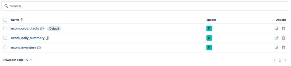
Create three data views:
ecom_order_facts with time field order_date_str, ecom_inventory with time field snapshot_ts, and ecom_daily_summary with time field sale_date.
After saving each one you can immediately explore data in the Discover tab, confirm that you can see order documents with all their enriched fields.
Alternatively, you can automate data view creation via the Kibana REST API. This is better for a reproducible pipeline:
create_data_views.sh
#!/bin/bash

KIBANA="http://localhost:5601"

echo "Creating ecom-order-facts data view..."

curl -s -X POST "$KIBANA/api/data_views/data_view" \
  -H "kbn-xsrf: true" \
  -H "Content-Type: application/json" \
  -d '{
    "data_view": {
      "id": "ecom-order-facts",
      "title": "ecom_order_facts",
      "timeFieldName": "order_date_str"
    }
  }' | python3 -m json.tool

echo ""

echo "Creating ecom-inventory data view..."

curl -s -X POST "$KIBANA/api/data_views/data_view" \
  -H "kbn-xsrf: true" \
  -H "Content-Type: application/json" \
  -d '{
    "data_view": {
      "id": "ecom-inventory",
      "title": "ecom_inventory",
      "timeFieldName": "snapshot_ts"
    }
  }' | python3 -m json.tool

echo ""

echo "Creating ecom-daily-summary data view..."

curl -s -X POST "$KIBANA/api/data_views/data_view" \
  -H "kbn-xsrf: true" \
  -H "Content-Type: application/json" \
  -d '{
    "data_view": {
      "id": "ecom-daily-summary",
      "title": "ecom_daily_summary",
      "timeFieldName": "sale_date"
    }
  }' | python3 -m json.tool

echo ""
echo "Done."
In Kibana go to Visualize Library → Create visualization → Lens. Drag
sale_date onto the X axis, set the aggregation to Date histogram → 1 day, then drag total_revenue onto the Y axis and set it to Sum. The visual editor is intuitive and takes about two minutes per chart.
Putting It All Together
The final step is a top-level orchestration script that runs the entire pipeline in the correct order, create mappings, run Spark, import the Kibana dashboard, and reports timing for each stage.In a production environment you would replace this script with a workflow scheduler such as Apache Airflow, Prefect, or Dagster, which add retry logic, alerting, and lineage tracking. For local development this shell-script-in-Python approach is perfectly adequate:
run_pipeline.py
"""
End-to-end orchestrator.
  1. Create / reset Elasticsearch index mappings
  2. Run the Spark pipeline (Postgres → ES)
  3. Import Kibana dashboard
"""
import time
import subprocess
import sys


def run_step(label: str, module: str) -> float:
    print(f"\n{'═'*60}")
    print(f"  {label}")
    print(f"{'═'*60}")
    t0 = time.time()
    result = subprocess.run(
        [sys.executable, module],
        capture_output=False,
    )
    elapsed = time.time() - t0
    if result.returncode != 0:
        print(f"\n✗ Step failed: {module} (exit {result.returncode})")
        sys.exit(1)
    print(f"\n  ✓ Completed in {elapsed:.1f}s")
    return elapsed


if __name__ == "__main__":
    total_start = time.time()

    t1 = run_step("STEP 1 ── Create Elasticsearch mappings", "es_mappings.py")
    t2 = run_step("STEP 2 ── Spark: Postgres → Elasticsearch", "pipeline.py")
    t3 = run_step("STEP 3 ── Import Kibana dashboard", "kibana_dashboard.py")

    total = time.time() - total_start
    print(f"\n{'═'*60}")
    print(f"  Pipeline complete!")
    print(f"  ES mappings:  {t1:.1f}s")
    print(f"  Spark job:    {t2:.1f}s")
    print(f"  Kibana setup: {t3:.1f}s")
    print(f"  Total:        {total:.1f}s")
    print(f"{'═'*60}")
    print(f"\n  → Kibana: http://localhost:5601/app/dashboards")
python run_pipeline.py. Once it completes, open Kibana, navigate to Dashboards, and open E-Commerce Analytics, Spark Pipeline. Set the time filter to Last 1 year to cover the full range of seed data.
You should see the daily revenue area chart populated across 365 days, the horizontal bar chart ranking categories by revenue, and the margin metrics broken down by region.
From here the analytical possibilities are open-ended. In the Discover tab you can run ad-hoc KQL (Kibana Query Language) queries such as
status:DELIVERED AND category_name:Smartphones AND region:WEST and see individual order line documents in milliseconds.
In Lens you can build a cohort analysis by dragging
tier and order_month into a data table to understand whether Gold-tier customers place larger orders in Q4. The ecom_inventory index lets you build an operations dashboard showing which products are below reorder point per warehouse, a view that would require a slow analytical query in Postgres but is instant in Elasticsearch.
Several things to harden before going to production: enable Elasticsearch security (
xpack.security.enabled=true) and generate TLS certificates; set es.net.ssl=true and es.net.ssl.cert.allow.self.signed=true (or provide proper certs) in the Spark config; configure ILM (Index Lifecycle Management) policies in Elasticsearch to roll over and retire old data automatically; replace the overwrite save mode in the Spark writer with append plus a proper es.mapping.id to achieve idempotent upserts; and containerise the Spark jobs themselves using the official apache/spark Docker image so the pipeline is deployable on Kubernetes or Amazon EMR.
The stack we have built, PostgreSQL 17.9 as the operational source of truth, PySpark 4.1 as the distributed transformation engine, Elasticsearch 9.4 as the analytical store, and Kibana 9.4 as the visualisation layer, represents a pattern that scales comfortably from gigabytes to petabytes with minimal architectural change.
The only things that change at scale are the number of Spark executors and the number of Elasticsearch shards. The code stays the same.
Project file structure
ecom-pipeline/
├── docker-compose.yml       ← PostgreSQL, Elasticsearch, Kibana
├── sql/
│   └── init.sql             ← Schema + seed data (auto-runs on pg boot)
├── jars/
│   └── postgresql-42.7.4.jar
├── spark_session.py         ← SparkSession factory + connection constants
├── read_postgres.py         ← JDBC reads (simple + partitioned)
├── transforms.py            ← Joins, aggregations, feature engineering
├── es_mappings.py           ← Create ES index mappings
├── pipeline.py              ← Main Spark → ES writer
├── kibana_dashboard.py      ← Saved objects import
├── explore.py               ← Exploratory queries (dev only)
├── create_data_views.sh     ← Creates Kibana Data Views automatically
└── run_pipeline.py          ← Top-level orchestrator
Running the Pipeline End-to-End
The commands below are the exact sequence validated on macOS with OpenJDK 17 installed via Homebrew.Step 1: Verify Transforms and Joins
python read_postgres.py
[read_postgres] Loading dimension tables …
.
.
.

── categories ──
+-----------+-------------+---------+
|category_id|name         |parent_id|
+-----------+-------------+---------+
|1          |Electronics  |NULL     |
|2          |Clothing     |NULL     |
|3          |Home & Garden|NULL     |
|4          |Sports       |NULL     |
|5          |Books        |NULL     |
+-----------+-------------+---------+
only showing top 5 rows

── products ──
+----------+-----------+------+--------------------+-------+-------+---------+--------------------------+
|product_id|category_id|sku   |name                |price  |cost   |is_active|created_at                |
+----------+-----------+------+--------------------+-------+-------+---------+--------------------------+
|1         |6          |SP-001|ProPhone 15 Ultra   |1099.00|620.00 |true     |2026-05-28 12:49:53.132774|
|2         |6          |SP-002|ProPhone 15 Standard|799.00 |420.00 |true     |2026-05-28 12:49:53.132774|
|3         |6          |SP-003|BudgetPhone Z1      |299.00 |140.00 |true     |2026-05-28 12:49:53.132774|
|4         |6          |SP-004|MidPhone X5         |549.00 |280.00 |true     |2026-05-28 12:49:53.132774|
|5         |7          |LP-001|DevBook Pro 16      |1899.00|1050.00|true     |2026-05-28 12:49:53.132774|
+----------+-----------+------+--------------------+-------+-------+---------+--------------------------+
only showing top 5 rows

── customers ──
+-----------+-----------------+----------+---------+-------+--------+--------------------------+
|customer_id|email            |first_name|last_name|region |tier    |registered_at             |
+-----------+-----------------+----------+---------+-------+--------+--------------------------+
|1          |user1@example.com|Bob       |Williams |SOUTH  |BRONZE  |2026-05-28 12:49:53.134217|
|2          |user2@example.com|Carol     |Evans    |EAST   |SILVER  |2026-05-28 12:49:53.134217|
|3          |user3@example.com|David     |Roberts  |WEST   |SILVER  |2026-05-28 12:49:53.134217|
|4          |user4@example.com|Eva       |Brown    |CENTRAL|GOLD    |2026-05-28 12:49:53.134217|
|5          |user5@example.com|Frank     |Davies   |NORTH  |PLATINUM|2026-05-28 12:49:53.134217|
+-----------+-----------------+----------+---------+-------+--------+--------------------------+
only showing top 5 rows

── inventory ──
+------------+----------+----------+-----------+-------------+-------------------------+
|inventory_id|product_id|warehouse |qty_on_hand|reorder_point|last_updated             |
+------------+----------+----------+-----------+-------------+-------------------------+
|1           |1         |WH-EAST   |69         |41           |2026-05-28 12:49:53.16403|
|2           |1         |WH-WEST   |370        |17           |2026-05-28 12:49:53.16403|
|3           |1         |WH-CENTRAL|299        |15           |2026-05-28 12:49:53.16403|
|4           |2         |WH-EAST   |212        |11           |2026-05-28 12:49:53.16403|
|5           |2         |WH-WEST   |79         |25           |2026-05-28 12:49:53.16403|
+------------+----------+----------+-----------+-------------+-------------------------+
only showing top 5 rows

── orders ──
+--------+-----------+---------+--------------------------+--------------------------+-----------+-----------+------------+
|order_id|customer_id|status   |order_date                |shipped_date              |channel    |coupon_code|discount_pct|
+--------+-----------+---------+--------------------------+--------------------------+-----------+-----------+------------+
|1       |2          |CONFIRMED|2026-04-21 01:16:05.168359|NULL                      |WEB        |NULL       |0.00        |
|2       |3          |SHIPPED  |2025-07-21 07:14:00.321576|2026-01-21 10:47:59.338759|MOBILE     |NULL       |5.00        |
|3       |4          |DELIVERED|2025-10-24 12:29:54.326842|2025-10-30 20:51:21.334158|MARKETPLACE|NULL       |10.00       |
|4       |5          |DELIVERED|2025-08-30 08:20:04.184441|2025-09-05 20:02:43.622241|RETAIL     |NULL       |15.00       |
|5       |6          |DELIVERED|2026-01-06 17:46:23.252496|2025-12-07 10:07:59.375032|WEB        |NULL       |20.00       |
+--------+-----------+---------+--------------------------+--------------------------+-----------+-----------+------------+
only showing top 5 rows

── order_items ──
+-------+--------+----------+--------+----------+
|item_id|order_id|product_id|quantity|unit_price|
+-------+--------+----------+--------+----------+
|1      |1       |2         |1       |79.00     |
|2      |1       |3         |1       |79.00     |
|3      |1       |4         |4       |79.00     |
|4      |2       |2         |2       |75.05     |
|5      |2       |3         |3       |75.05     |
+-------+--------+----------+--------+----------+
only showing top 5 rows
Step 2: Validate Joins and Aggregations
python explore.py
[read_postgres] Loading dimension tables …
[read_postgres] Loading fact tables with partitioning …
.
.
.

── Top 5 Categories by Revenue ─────────────────
+-------------+---------+
|category_name|  revenue|
+-------------+---------+
|  Smartphones|289009.65|
|      Laptops| 48881.25|
+-------------+---------+


── Revenue by Region and Channel ───────────────
+-------+-----------+--------+------+
| region|    channel| revenue|orders|
+-------+-----------+--------+------+
|CENTRAL|MARKETPLACE|41613.25|    75|
|   EAST|        WEB|39322.25|    75|
|  NORTH|     RETAIL|39906.85|    75|
|  SOUTH|        WEB|41435.50|    75|
|   WEST|     MOBILE|40898.30|    75|
+-------+-----------+--------+------+


── Null check on key columns ───────────────────
  order_id              nulls: 0
  product_id            nulls: 0
  customer_id           nulls: 0
  category_name         nulls: 0
  region                nulls: 0
  line_revenue          nulls: 0

── Low-stock products ──────────────────────────
+----------------+---------+-----------+-------------+------------+
|product_name    |warehouse|qty_on_hand|reorder_point|stock_status|
+----------------+---------+-----------+-------------+------------+
|Classic Crew Tee|WH-EAST  |14         |50           |LOW_STOCK   |
+----------------+---------+-----------+-------------+------------+
Step 3: Create Elasticsearch Index mappings
python es_mappings.pyCreated index 'ecom_order_facts'
Created index 'ecom_inventory'
Created index 'ecom_daily_summary'
All indices created. Run pipeline.py next.
Step 4: Run the Spark Pipeline (Postgres → Elasticsearch)
python pipeline.py
.
.
.
.
══ Step 1 / 4 ── Reading from PostgreSQL ════════════════
[read_postgres] Loading dimension tables …
[read_postgres] Loading fact tables with partitioning …
  categories           12 rows  |  schema: [('category_id', 'int'), ('name', 'string'), ('parent_id', 'int')]
  products             30 rows  |  schema: [('product_id', 'int'), ('category_id', 'int'), ('sku', 'string'), ('name', 'string'), ('price', 'decimal(10,2)'), ('cost', 'decimal(10,2)'), ('is_active', 'boolean'), ('created_at', 'timestamp')]
  customers           200 rows  |  schema: [('customer_id', 'int'), ('email', 'string'), ('first_name', 'string'), ('last_name', 'string'), ('region', 'string'), ('tier', 'string'), ('registered_at', 'timestamp')]
  inventory            90 rows  |  schema: [('inventory_id', 'int'), ('product_id', 'int'), ('warehouse', 'string'), ('qty_on_hand', 'int'), ('reorder_point', 'int'), ('last_updated', 'timestamp')]
  orders            1,000 rows  |  schema: [('order_id', 'int'), ('customer_id', 'int'), ('status', 'string'), ('order_date', 'timestamp'), ('shipped_date', 'timestamp'), ('channel', 'string'), ('coupon_code', 'string'), ('discount_pct', 'decimal(5,2)')]
  order_items       3,000 rows  |  schema: [('item_id', 'int'), ('order_id', 'int'), ('product_id', 'int'), ('quantity', 'int'), ('unit_price', 'decimal(10,2)')]

══ Step 2 / 4 ── Building Spark DataFrames ══════════════
  order_facts rows: 3,000
  inventory_snap rows: 90
  daily_summary rows: 712

══ Step 3 / 4 ── Writing to Elasticsearch ═══════════════
  ✓ Written → ecom_order_facts
  ✓ Written → ecom_inventory
  ✓ Written → ecom_daily_summary

══ Step 4 / 4 ── Done ═══════════════════════════════════
  Total time: 5.4s
Step 5: verify documents landed in elasticsearch
curl -s "http://localhost:9200/ecom_order_facts/_count"   | python3 -m json.tool
curl -s "http://localhost:9200/ecom_inventory/_count"     | python3 -m json.tool
curl -s "http://localhost:9200/ecom_daily_summary/_count" | python3 -m json.tool
{
    "count": 3000,
    "_shards": {
        "total": 2,
        "successful": 2,
        "skipped": 0,
        "failed": 0
    }
}
{
    "count": 90,
    "_shards": {
        "total": 1,
        "successful": 1,
        "skipped": 0,
        "failed": 0
    }
}
{
    "count": 712,
    "_shards": {
        "total": 1,
        "successful": 1,
        "skipped": 0,
        "failed": 0
    }
}
Step 6: Create Kibana Data View (Index Pattern)
bash create_data_views.shStep 7: Creating Kibana Dashboards and Visualizations
After the Elasticsearch indices and Data Views are ready, dashboards can be created in Kibana using Kibana Lens. Navigate to:Analytics → Visualize Library → Create Visualization → Lens Analytics → Dashboard → Create Dashboard