Learn Seaborn Visualization Basics

Seaborn is a powerful Python library built on top of Matplotlib that provides a high-level interface for creating attractive and informative statistical visualizations. It simplifies complex plotting tasks and offers beautiful default styles, making it a favorite tool for data analysis and exploratory data analysis (EDA).

1. Introduction to Seaborn

Seaborn is specifically designed for statistical data visualization. It integrates closely with Pandas DataFrames and supports complex visualizations with minimal code.

Key Features:

- Built-in themes and color palettes
- Easy handling of categorical data
- Advanced statistical plotting
- Seamless integration with Pandas
- Simplified syntax compared to Matplotlib

2. Installation

You can install Seaborn using pip:

pip install seaborn

3. Importing Libraries

import seaborn as sns
import matplotlib.pyplot as plt

4. Built-in Datasets

Seaborn provides several built-in datasets for practice.

df = sns.load_dataset('tips')
print(df.head())

Common datasets:

- tips
- iris
- titanic
- flights

5. Basic Plot: Scatter Plot

import seaborn as sns
import matplotlib.pyplot as plt

df = sns.load_dataset('tips')
print(df.head())

sns.scatterplot(x='total_bill', y='tip', data=df)
plt.show()

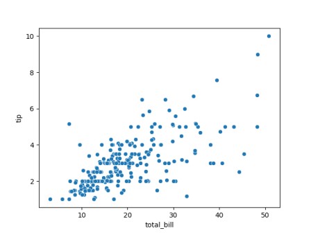
Output:

   total_bill   tip     sex smoker  day    time  size
0       16.99  1.01  Female     No  Sun  Dinner     2
1       10.34  1.66    Male     No  Sun  Dinner     3
2       21.01  3.50    Male     No  Sun  Dinner     3
3       23.68  3.31    Male     No  Sun  Dinner     2
4       24.59  3.61  Female     No  Sun  Dinner     4

Use Case:

Identify relationships between variables

6. Line Plot

import seaborn as sns
import matplotlib.pyplot as plt

df = sns.load_dataset('tips')
print(df.head())

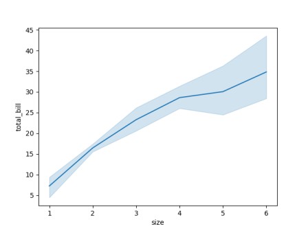
sns.lineplot(x='size', y='total_bill', data=df)
plt.show()

Output:

   total_bill   tip     sex smoker  day    time  size
0       16.99  1.01  Female     No  Sun  Dinner     2
1       10.34  1.66    Male     No  Sun  Dinner     3
2       21.01  3.50    Male     No  Sun  Dinner     3
3       23.68  3.31    Male     No  Sun  Dinner     2
4       24.59  3.61  Female     No  Sun  Dinner     4

Use Case:

Trend analysis

7. Bar Plot

import seaborn as sns
import matplotlib.pyplot as plt

df = sns.load_dataset('tips')
print(df.head())

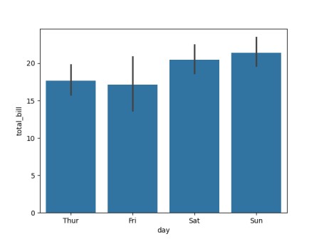
sns.barplot(x='day', y='total_bill', data=df)
plt.show()

Output:

   total_bill   tip     sex smoker  day    time  size
0       16.99  1.01  Female     No  Sun  Dinner     2
1       10.34  1.66    Male     No  Sun  Dinner     3
2       21.01  3.50    Male     No  Sun  Dinner     3
3       23.68  3.31    Male     No  Sun  Dinner     2
4       24.59  3.61  Female     No  Sun  Dinner     4

Features:

- Automatically calculates mean values
- Shows confidence intervals

8. Histogram and Distribution Plot

import seaborn as sns
import matplotlib.pyplot as plt

df = sns.load_dataset('tips')
print(df.head())

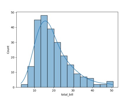
sns.histplot(df['total_bill'], kde=True)
plt.show()

Output:

   total_bill   tip     sex smoker  day    time  size
0       16.99  1.01  Female     No  Sun  Dinner     2
1       10.34  1.66    Male     No  Sun  Dinner     3
2       21.01  3.50    Male     No  Sun  Dinner     3
3       23.68  3.31    Male     No  Sun  Dinner     2
4       24.59  3.61  Female     No  Sun  Dinner     4

Key Concepts:

- Distribution of data
- KDE (Kernel Density Estimation)

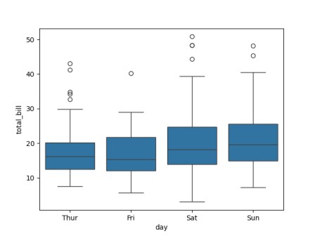
9. Box Plot

import seaborn as sns
import matplotlib.pyplot as plt

df = sns.load_dataset('tips')
print(df.head())

sns.boxplot(x='day', y='total_bill', data=df)
plt.show()

Output:

   total_bill   tip     sex smoker  day    time  size
0       16.99  1.01  Female     No  Sun  Dinner     2
1       10.34  1.66    Male     No  Sun  Dinner     3
2       21.01  3.50    Male     No  Sun  Dinner     3
3       23.68  3.31    Male     No  Sun  Dinner     2
4       24.59  3.61  Female     No  Sun  Dinner     4

Use Case:

- Detect outliers
- Understand data spread

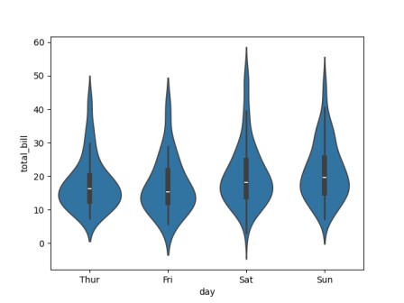
10. Violin Plot

import seaborn as sns
import matplotlib.pyplot as plt

df = sns.load_dataset('tips')
print(df.head())

sns.violinplot(x='day', y='total_bill', data=df)
plt.show()

Output:

   total_bill   tip     sex smoker  day    time  size
0       16.99  1.01  Female     No  Sun  Dinner     2
1       10.34  1.66    Male     No  Sun  Dinner     3
2       21.01  3.50    Male     No  Sun  Dinner     3
3       23.68  3.31    Male     No  Sun  Dinner     2
4       24.59  3.61  Female     No  Sun  Dinner     4

Advantage:

Combines box plot and distribution

11. Pair Plot

import seaborn as sns
import matplotlib.pyplot as plt

df = sns.load_dataset('tips')
print(df.head())

sns.pairplot(df)
plt.show()

Output:

   total_bill   tip     sex smoker  day    time  size
0       16.99  1.01  Female     No  Sun  Dinner     2
1       10.34  1.66    Male     No  Sun  Dinner     3
2       21.01  3.50    Male     No  Sun  Dinner     3
3       23.68  3.31    Male     No  Sun  Dinner     2
4       24.59  3.61  Female     No  Sun  Dinner     4

Use Case:

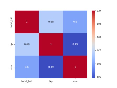
Visualize relationships across multiple variables

12. Heatmap

import seaborn as sns
import matplotlib.pyplot as plt

df = sns.load_dataset('tips')
print(df.head())

corr = df.corr(numeric_only=True)
sns.heatmap(corr, annot=True, cmap='coolwarm')
plt.show()

Output:

    total_bill   tip     sex smoker  day    time  size
0       16.99  1.01  Female     No  Sun  Dinner     2
1       10.34  1.66    Male     No  Sun  Dinner     3
2       21.01  3.50    Male     No  Sun  Dinner     3
3       23.68  3.31    Male     No  Sun  Dinner     2
4       24.59  3.61  Female     No  Sun  Dinner     4

Use Case:

Display correlation matrix

13. Customization in Seaborn

Themes

sns.set_style("darkgrid")

Available styles:

- white
- dark
- whitegrid
- darkgrid
- ticks

Color Palettes

sns.set_palette("pastel")

Popular palettes:

- deep
- muted
- bright
- pastel

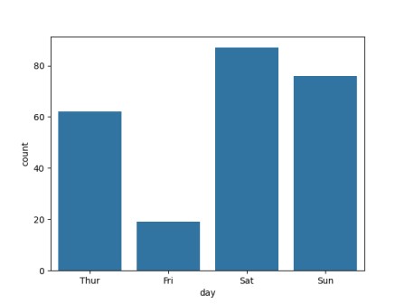
14. Working with Categorical Data

import seaborn as sns
import matplotlib.pyplot as plt

df = sns.load_dataset('tips')
print(df.head())

sns.countplot(x='day', data=df)
plt.show()

Output:

   total_bill   tip     sex smoker  day    time  size
0       16.99  1.01  Female     No  Sun  Dinner     2
1       10.34  1.66    Male     No  Sun  Dinner     3
2       21.01  3.50    Male     No  Sun  Dinner     3
3       23.68  3.31    Male     No  Sun  Dinner     2
4       24.59  3.61  Female     No  Sun  Dinner     4

Use Case:

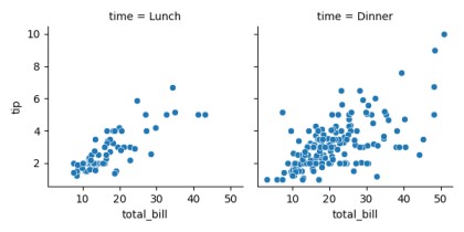
Count occurrences of categories

15. FacetGrid (Advanced)

import seaborn as sns
import matplotlib.pyplot as plt

df = sns.load_dataset('tips')
print(df.head())

g = sns.FacetGrid(df, col="time")
g.map(sns.scatterplot, "total_bill", "tip")
plt.show()

Output:

   total_bill   tip     sex smoker  day    time  size
0       16.99  1.01  Female     No  Sun  Dinner     2
1       10.34  1.66    Male     No  Sun  Dinner     3
2       21.01  3.50    Male     No  Sun  Dinner     3
3       23.68  3.31    Male     No  Sun  Dinner     2
4       24.59  3.61  Female     No  Sun  Dinner     4

Use Case:

Multi-plot visualization by categories

16. Advantages of Seaborn

- Simple syntax for complex visualizations
- Built-in support for statistical analysis
- Attractive default designs
- Tight integration with Pandas

17. Limitations of Seaborn

- Less control compared to Matplotlib
- Limited for highly customized plots
- Depends on Matplotlib backend

18. Best Practices

- Choose the right plot type for your data
- Use color wisely to highlight insights
- Avoid clutter and over-plotting
- Always label axes and titles
- Combine Seaborn with Matplotlib for customization

19. Seaborn vs Matplotlib

Feature	Seaborn	Matplotlib
Level	High-level	Low-level
Ease of Use	Easy	Moderate
Default Styling	Attractive	Basic
Flexibility	Moderate	High

Seaborn is an essential tool for anyone involved in data science or data analysis. It simplifies the process of creating complex statistical visualizations and enhances the visual appeal of your plots.

Learn Seaborn Visualization Basics

1. Introduction to Seaborn

Key Features:

2. Installation

3. Importing Libraries

4. Built-in Datasets

Common datasets:

5. Basic Plot: Scatter Plot

Output:

Use Case:

6. Line Plot

Output:

Use Case:

7. Bar Plot

Output:

Features:

8. Histogram and Distribution Plot

Output:

Key Concepts:

9. Box Plot

Output:

Use Case:

10. Violin Plot

Output:

Advantage:

11. Pair Plot

Output:

Use Case:

12. Heatmap

Output:

Use Case:

13. Customization in Seaborn

Themes

Available styles:

Color Palettes

Popular palettes:

14. Working with Categorical Data

Output:

Use Case:

15. FacetGrid (Advanced)

Output:

Use Case:

16. Advantages of Seaborn

17. Limitations of Seaborn

18. Best Practices

19. Seaborn vs Matplotlib

Nagesh Chauhan

Share this Article

💬 Comments

Join the discussion